Coursework
CSci 39542: Introduction to Data Science
Department of Computer Science
Hunter College, City University of New York
Fall 2023
Classwork Midterm Exam Programming Assignments Project Final Exam
All students registered by Wednesday, 23 August are sent a Gradescope registration invitation to the email on record on their Blackboard account. If you did not receive the email or would like to use a different account, write to datasci@hunter.cuny.edu. Include in your email that you not receive a Gradescope invitation, your preferred email, and your EmpID. We will manually generate an invitation. As a default, we use your name as it appears in Blackboard/CUNYFirst (to update CUNYFirst, see changing your personal information). If you prefer a different name for Gradescope, include it, and we will update the Gradescope registration.
Classwork
Unless otherwise noted, classwork is submitted via Gradescope.
Access information is given during the corresponding lecture.
To get the most out of lecture, bring a device with you to lecture with a development environment (IDE) that has Python 3+ (preferrably the same that you plan to use for technical interviews).
Note: Hunter College is committed to all students having the technology needed for their courses. If you are in need of technology, see
Student Life's Support & Resources Page.
If you attended class that day, there is an option to earn 0.5 points for attendance for each part of lecture. and space to include the row and seat number. If you were not able to attend a given lecture, you can still work through the classwork at home and we will replace the fractional point for that classwork with the grade you earned on the final exam.
Do not say you were in the room if you did not attend. Lying about attendance obtains an unfair advantage and will be submitted to the Office of Student Conduct. It is not worth 0.5 points (that would have been replaced anyway by your final exam score) for a record of academic dishonesty that is kept by both the department and college. The suggested sanction for lying is a 0 on this classwork and the loss of the replacement policy for missed lecture grades. Note: while we suggest a sanction, the final decision about the severity of the sanction is by the Office of Student Conduct.
- Week 0:
Classwork 0: Due midnight, Tuesday, 29 August. Available on Wednesday, 23 August, this classwork focuses on the course syllabus and frequently asked questions.
- Week 1:
Classwork 1.1: Due 1:45pm, Wednesday, 30 August. Available during Lecture 1 on Gradescope, this classwork introduces the autograder that is used for the programming assignments. The structure of the sample program mirrors the structure and content of the upcoming Program 1 (which we will start in the second part of Lecture 1).
Write a function that takes the name of a file and makes a dictionary of the lines of the file.
-
make_dict(file_name, sep=': '): Takes a name of a file,file_nameand a delimitersep. The default value is': '. If a line of the file does not includesep, the line should be ignored. Otherwise, for each line, the string preceding the delimitersepis the key, and the string aftersepis the value. Your function returns the dictionary.
For example, assuming these functions are in a file,
cw1.pyand run on a file containing names that start with 'A', contacts.txt:
will print:contacts = cw1.make_dict('contacts.txt') who = 'CS Department' print(f'Contact info for {who} is {contacts[who]}.')Contact info for CS Department is 10th Floor HN, x5213.Another example with nick_names.txt:
will print:nick_names = cw1.make_dict('nick_names.txt', sep = ' ') names = ['Beth','Lisa','Meg','Greta','Amy','Mia'] for n in names: print(f'Full name for {n} is {nick_names[n]}.')Full name for Beth is Elizabeth. Full name for Lisa is Elizabeth. Full name for Meg is Margaret. Full name for Greta is Margaret. Full name for Amy is Amelia. Full name for Mia is Amelia.If you attended lecture, include the last line to the introductory comment:
If you did not attend lecture, do not include the last line.""" Name: YOUR_NAME Email: YOUR_EMAIL Resources: RESOURCES USED I attended lecture today. """Classwork 1.2: Due 3pm, Wednesday, 30 August. In the second part of Lecture 1, we will start Program 1. At the end of lecture, having a positive score on the first program gives credit for this classwork. You do not need to complete the first program or submit anything extra, we will generate the scores directly by if you have submitted an attempt to Gradescope.
-
- Week 2:
Classwork 2.1: Due 1:45pm, Wednesday, 6 September. Available during Lecture 2 on Gradescope, this classwork asks that you write a program using Pandas and its file I/O. To get the most out of this exercise, bring a laptop with you to lecture with a development environment (IDE) that has Python 3.6+ to work through in lecture.
Write a program that asks the user for the name of an input CSV file and the name of an output CSV file. The program should open the file name provided by the user. Next, the program should select rows where the field
Gradeis equal to 3 and theYearis equal to 2019 and write all rows that match that criteria to a new CSV file.Then a sample run of the program:
where the fileEnter input file name: school-ela-results-2013-2019.csv Enter output file name: ela2013.csvschool-ela-results-2013-2019.csvis extracted from NYC Schools Test Results (and truncated version of roughly the first 1000 lines for testing). The first lines of the output file would be:School,Name,Grade,Year,Category,Number Tested,Mean Scale Score,# Level 1,% Level 1,# Level 2,% Level 2,# Level 3,% Level 3,# Level 4,% Level 4,# Level 3+4,% Level 3+4 01M015,P.S. 015 ROBERTO CLEMENTE,3,2019,All Students,27,606,1,3.7,7,25.9,18,66.7,1,3.7,19,70.4 01M019, P.S. 019 ASHER LEVY,3,2019,All Students,24,606,0,0.0,8,33.3,15,62.5,1,4.2,16,66.7 01M020,P.S. 020 ANNA SILVER,3,2019,All Students,57,593,13,22.8,24,42.1,18,31.6,2,3.5,20,35.1Hints:
- Since the
Gradecolumn contains a mixtures of numbers (e.g. 3) and strings ("All Grades"), the column is stored as strings.
If you attended lecture, include the last line to the introductory comment:
If you did not attend lecture, do not include the above lines.""" Name: YOUR_NAME Email: YOUR_EMAIL Resources: RESOURCES USED I attended lecture today. """Classwork 2.2: Due 3pm, Wednesday, 6 September. Complete as much as possible of the HackerRank Challenge: Map & Lambda Expressions. Fill in with comments where you got stuck and what you would do with more time. Copy your commented code to the Classwork 2.2 in Gradescope.
- Since the
- Week 3:
Classwork 3.1: Due 1:45pm, Wednesday, 13 September. In the first part of Lecture 3, we will start Program 2. Having successfully started the second program to Gradescope (i.e. a positive score) by the end of break gives credit for this classwork. You do not need to complete the second program or submit anything extra, we will generate the scores directly by if you have submitted an attempt to Gradescope.
Classwork 3.2: Due 3pm, Wednesday, 13 September. The second part of the classwork focuses on linear regression and is on paper. To receive credit, make sure to turn in your paper with your name and EmpID by the end of lecture.
- Week 4:
Classwork 4.1: Due 1:45pm, Wednesday, 20 September. Available during Lecture 4 on Gradescope, this classwork focuses on hiring in the technical sector. Last fall, hiring looked quite strong. Here's a an analysis by Prof. Stevenson of University of Michigan:

BLS Monthly Jobs Report: Rapid Insights from Betsey Stevenson.Including more recent numbers show growth but not as quickly:
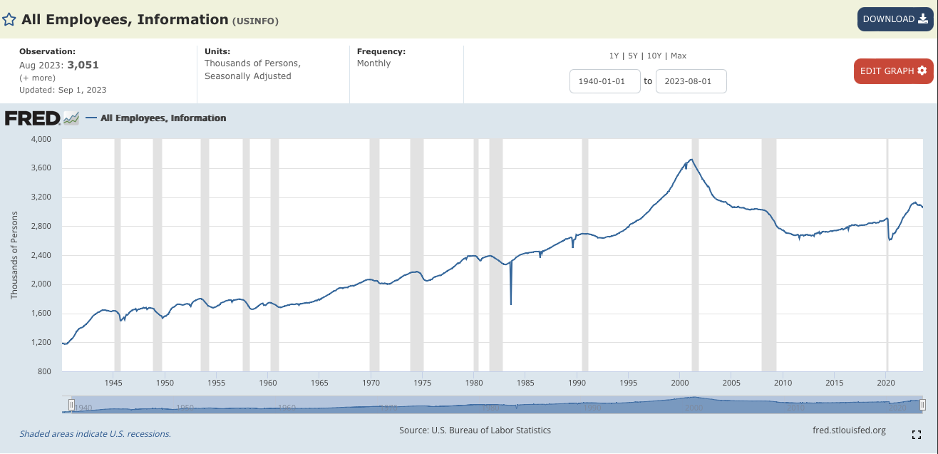
Available Libraries: pandas, numpy, sklearn.linear_model, pickle.
Using the data set for 2010 until August 2023 from St. Louis Federal Reserve Economic Data Data (FRED):
- fred_info_2010_aug_2023.csv: A CSV file with the employment in Information Services since 2010 (until August 2023).
-
fit_linear_regression(df)This function takes one input:-
df: containing an index and the column,USINFO.
indexand????, usingsklearn.linear_model.LinearRegression(see lecture & textbook for details on setting up the model). The resulting model should be returned as bytestream, using pickle (see Lecture 4).
Hint: Since each entry is exactly 1 month apart, you can use the index, instead of parsing thedatetimeobjects. You may finddf.index.to_series()useful. -
-
predict(mod_pkl, offset):This function takes two inputs:-
mod_pkl: a trained model for the data, stored in pickle format. -
offset: the number of months since January 1, 2010.
mod_pkl, returns the predicted number of employees in Information Servicesoffsetmonths from January 1, 2010. For example ifoffsetis180, then it would return the model's prediction of the number of employees180/12 = 15years after the baseline (January 2010) or January 2025. -
For example:
df = pd.read_csv(directory+'fred_info_2010_aug_2023.csv')
mod_pkl = fit_linear_regression(df)
januarys = pd.DataFrame({'index' : list(range(120,240,12))})
predictions = predict(mod_pkl,januarys)
print(f'The predicted employments by years:')
results = zip(list(range(2020,2030)),predictions)
for year,pred in results:
print(f'January {year}: \t {int(pred*1000):,}')The predicted employments by years:
January 2020: 2,879,867
January 2021: 2,905,173
January 2022: 2,930,480
January 2023: 2,955,786
January 2024: 2,981,092
January 2025: 3,006,398
January 2026: 3,031,705
January 2027: 3,057,011
January 2028: 3,082,317
January 2029: 3,107,623Classwork 4.2: Due 3pm, Wednesday, 20 September. Available during Lecture 4 on Gradescope, this classwork focuses on the structure and topics for the optional project, based on the project overview in lecture:
- What is an NYC-related topic in which you are interested?
- Was is a question related to that topic (i.e. predictive instead of descriptive framing of your project)?
- What kind of data would you be needed for this?
Classwork 5.1: Due 1:45pm, Wednesday, 27 September. In the first part of Lecture 5, we will start Program 3. Having successfully started the third program to Gradescope (i.e. a positive score) by the end of break gives credit for this classwork. You do not need to complete the thid program or submit anything extra, we will generate the scores directly by if you have submitted an attempt to Gradescope.
Classwork 5.2: Due 3pm, Wednesday, 27 September. The second part of the classwork focuses on Voronoi diagrams and is on Gradescope. To receive credit, make sure to submit the on-line Gradescope classwork by the end of lecture.
Classwork 6.1: Due 1:45pm, Wednesday, 4 October. Available during Lecture 6 on Gradescope, the learning objective of this classwork is to increase understanding of smoothing and gain fluidity with using distributions for smoothing. To get the most out of this exercise, bring a laptop with you to lecture with a development environment (IDE) that has Python 3.6+ to work through in lecture.
In Lecture 5 and Section 11.2, we used smoothing to visualize data. For this program, write a function that takes two arguments, an Numpy array of x-axis coordinates, and a list of numeric values, and returns the corresponding y-values for the sum of the gaussian probability distribution functions (pdf's) for each point in the list.
-
computeSmoothing(xes,points): This function takes a numpy arrayxesand a list,points, of numeric values. For eachpinpoints, the function should compute the normal probability distribution function (scipy.norm.pdf) centered atloc = pwith standard deviationscale = 0.5for all values inxes. The return value is a numpy array of the sum of these at each point.
For example, calling the function:
xes = np.linspace(0, 10, 1000)
density = computeSmoothing(xes,[5])
plt.plot(xes,density)
plt.show()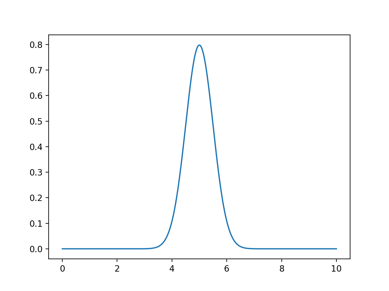
since there is only one point given (namely 5), the returned value is the probability density function centered at 5 (with scale = 0.5) computed for each of the xes.
For example, calling the function:
pts = [2,2,5,5,2,3,4,6,7,9]
xes = np.linspace(0, 10, 1000)
density = computeSmoothing(xes,pts)
plt.plot(xes,density)
plt.fill_between(xes,density)
plt.show()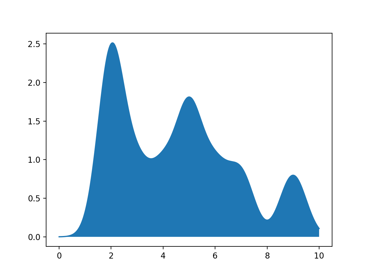
since the there are 10 points given, the function computes the probability density function centered at each of the points, across all the values in xes. It then sums up these contributions and returns an array of the same length as xes.
Note: you should submit a file with only the standard comments at the top, and this function. The grading scripts will then import the file for testing. If you attended lecture, include in the introductory comment the three lines detailed in Classwork 2.
Classwork 6.2: Due 3pm, Wednesday, 4 October. The second classwork for today's lecture is a practice runthrough of the exam & exam seating. We will use the seating chart of the exam to make sure everyone knows where their seat is (roughly alphabetical by first name). Credit for this classwork is given for the signed seating slip is picked up during the mock exam.
Classwork 7.1: Signed seating slip is picked up during the written portion of the exam.
Classwork 7.2: Signed seating slip is picked up during the coding portion of the exam.
Classwork 8.1: Due 1:45pm, Wednesday, 18 October. Available during Lecture 8 on Gradescope, this classwork introduces the canonical digits dataset and uses sci-kit learn to build logistic regression models. To get the most out of this exercise, bring a laptop with you to lecture with a development environment (IDE) that has Python 3+ to work through in lecture.
This program uses the canonical MNIST dataset of hand-written digits and available in sklearn digits dataset:
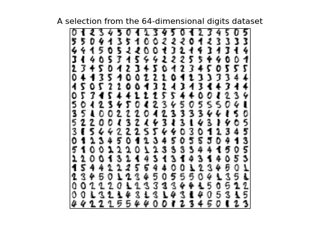
The dataset has 1797 scans of hand-written digits.
Each entry has the digit represented (target) as well as the 64 values representing the gray scale for the 8 x 8 image. The first 5 entries are:

The gray scales for the first 5 entries, flattened to one dimensional array:
[[ 0.  0.  5. 13.  9.  1.  0.  0.  0.  0. 13. 15. 10. 15.  5.  0.  0.  3. 15.  2.  0. 11.  8.  0.  0.  4. 12.  0.  0.  8.  8.  0.  0.  5.  8.  0.  0.  9.  8.  0.  0.  4. 11.  0.  1. 12.  7.  0.  0.  2. 14.  5. 10. 12.  0.  0.  0.  0.  6. 13. 10.  0.  0.  0.]
 [ 0.  0.  0. 12. 13.  5.  0.  0.  0.  0.  0. 11. 16.  9.  0.  0.  0.  0.  3. 15. 16.  6.  0.  0.  0.  7. 15. 16. 16.  2.  0.  0.  0.  0.  1. 16. 16.  3.  0.  0.  0.  0.  1. 16. 16.  6.  0.  0.  0.  0.  1. 16. 16.  6.  0.  0.  0.  0.  0. 11. 16. 10.  0.  0.]
 [ 0.  0.  0.  4. 15. 12.  0.  0.  0.  0.  3. 16. 15. 14.  0.  0.  0.  0.  8. 13.  8. 16.  0.  0.  0.  0.  1.  6. 15. 11.  0.  0.  0.  1.  8. 13. 15.  1.  0.  0.  0.  9. 16. 16.  5.  0.  0.  0.  0.  3. 13. 16. 16. 11.  5.  0.  0.  0.  0.  3. 11. 16.  9.  0.]
 [ 0.  0.  7. 15. 13.  1.  0.  0.  0.  8. 13.  6. 15.  4.  0.  0.  0.  2.  1. 13. 13.  0.  0.  0.  0.  0.  2. 15. 11.  1.  0.  0.  0.  0.  0.  1. 12. 12.  1.  0.  0.  0.  0.  0.  1. 10.  8.  0.  0.  0.  8.  4.  5. 14.  9.  0.  0.  0.  7. 13. 13.  9.  0.  0.]
 [ 0.  0.  0.  1. 11.  0.  0.  0.  0.  0.  0.  7.  8.  0.  0.  0.  0.  0.  1. 13.  6.  2.  2.  0.  0.  0.  7. 15.  0.  9.  8.  0.  0.  5. 16. 10.  0. 16.  6.  0.  0.  4. 15. 16. 13. 16.  1.  0.  0.  0.  0.  3. 15. 10.  0.  0.  0.  0.  0.  2. 16.  4.  0.  0.]]
Today, we will focus on entries that represent 0's and 1's. The first 10 from the dataset are displayed below:

Write a function that builds a logistic regression model that classifies binary digits:
-
def binary_digit_clf(data, target, test_size = 0.25, random_state = 21):: This function has four inputs:-
data: a numpy array that includes rows of equal size flattend arrays, -
targeta numpy array that takes values 0 or 1 corresponding to the rows ofdata. -
test_size: the size of the test set created when the data is divided into test and training sets with train_test_split. The default value is0.25. -
random_state: the random seed used when the data is divided into test and training sets with train_test_split. The default value is21.
-
For example, let's flatten the entries and restrict the dataset to just binary digits:
#Import datasets, classifiers and performance metrics:
from sklearn import datasets, svm, metrics
from sklearn.model_selection import train_test_split
from sklearn.linear_model import LogisticRegression
#Using the digits data set from sklearn:
from sklearn import datasets
digits = datasets.load_digits()
print(digits.target)
print(type(digits.target), type(digits.data))
#flatten the images
n_samples = len(digits.images)
data = digits.images.reshape((n_samples, -1))
print(data[0:5])
print(f'The targets for the first 5 entries: {digits.target[:5]}')
#Make a DataFrame with just the binary digits:
binaryDigits = [(d,t) for (d,t) in zip(data,digits.target) if t <= 1]
bd,bt = zip(*binaryDigits)
print(f'The targets for the first 5 binary entries: {bt[:5]}')
[0 1 2 ... 8 9 8]

[[ 0.  0.  5. 13.  9.  1.  0.  0.  0.  0. 13. 15. 10. 15.  5.  0.  0.  3.
15.  2.  0. 11.  8.  0.  0.  4. 12.  0.  0.  8.  8.  0.  0.  5.  8.  0.
0.  9.  8.  0.  0.  4. 11.  0.  1. 12.  7.  0.  0.  2. 14.  5. 10. 12.
0.  0.  0.  0.  6. 13. 10.  0.  0.  0.]
 [ 0.  0.  0. 12. 13.  5.  0.  0.  0.  0.  0. 11. 16.  9.  0.  0.  0.  0.
3. 15. 16.  6.  0.  0.  0.  7. 15. 16. 16.  2.  0.  0.  0.  0.  1. 16.
16.  3.  0.  0.  0.  0.  1. 16. 16.  6.  0.  0.  0.  0.  1. 16. 16.  6.
0.  0.  0.  0.  0. 11. 16. 10.  0.  0.]
 [ 0.  0.  0.  4. 15. 12.  0.  0.  0.  0.  3. 16. 15. 14.  0.  0.  0.  0.
8. 13.  8. 16.  0.  0.  0.  0.  1.  6. 15. 11.  0.  0.  0.  1.  8. 13.
15.  1.  0.  0.  0.  9. 16. 16.  5.  0.  0.  0.  0.  3. 13. 16. 16. 11.
5.  0.  0.  0.  0.  3. 11. 16.  9.  0.]
 [ 0.  0.  7. 15. 13.  1.  0.  0.  0.  8. 13.  6. 15.  4.  0.  0.  0.  2.
1. 13. 13.  0.  0.  0.  0.  0.  2. 15. 11.  1.  0.  0.  0.  0.  0.  1.
12. 12.  1.  0.  0.  0.  0.  0.  1. 10.  8.  0.  0.  0.  8.  4.  5. 14.
9.  0.  0.  0.  7. 13. 13.  9.  0.  0.]
 [ 0.  0.  0.  1. 11.  0.  0.  0.  0.  0.  0.  7.  8.  0.  0.  0.  0.  0.
1. 13.  6.  2.  2.  0.  0.  0.  7. 15.  0.  9.  8.  0.  0.  5. 16. 10.
0. 16.  6.  0.  0.  4. 15. 16. 13. 16.  1.  0.  0.  0.  0.  3. 15. 10.
0.  0.  0.  0.  0.  2. 16.  4.  0.  0.]]
The targets for the first 5 entries: [0 1 2 3 4]
The targets for the first 5 binary entries: (0, 1, 0, 1, 0)
We can then use the restricted data and targets datasets as input to our function, assuming your function binary_digit_clf():
confuse_mx = binary_digit_clf(bd,bt,test_size=0.95)
print(f'Confusion matrix:\n{confuse_mx}')
disp = metrics.ConfusionMatrixDisplay(confusion_matrix=confuse_mx)
#Use a different color map since the default is garish:
disp.plot(cmap = "Purples")
plt.title("Logistic Regression Classifier for Binary Digits")
plt.show()Confusion matrix:
[[172 0]
[ 4 166]]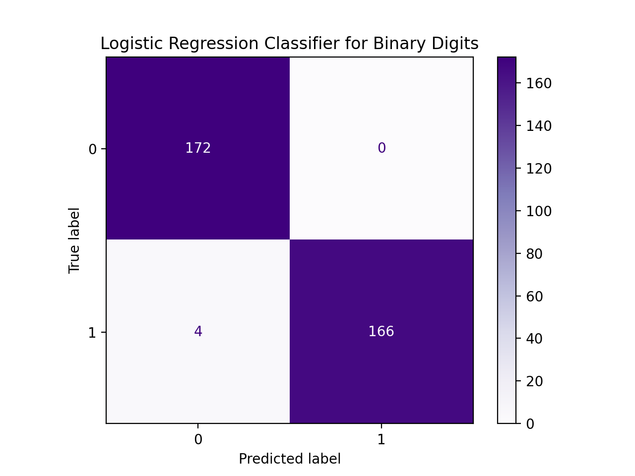
Another example with the same data, but different size for the data reserved for testing:
confuse_mx = binary_digit_clf(bd,bt)
print(f'Confusion matrix:\n{confuse_mx}')Confusion matrix:
[[43 0]
[ 0 47]]Note: you should submit a file with only the standard comments at the top, and this function. The grading scripts will then import the file for testing. If you attended lecture, include in the introductory comment the three lines detailed in Classwork 2.
Classwork 8.2: Due 3pm, Wednesday, 18 October. Available during Lecture 8 on Gradescope, this classwork recaps linear algebra.
Classwork 9.1: Due 1:45pm, Wednesday, 25 October. In the first part of Lecture 9, we will start Program 4. Having successfully started the fourth program to Gradescope (i.e. a positive score) by the end of break gives credit for this classwork. You do not need to complete the thid program or submit anything extra, we will generate the scores directly by if you have submitted an attempt to Gradescope.
Classwork 9.2: Due 3pm, Wednesday, 25 October.
We introduced Principal Components Analysis and the number of components needed to capture the intrinistic dimension of the data set. For this program, write a function that allows the user to explore how many dimensions are needed to see the underlying structure of images from the sklearn digits dataset (inspired by Python Data Science Handbook: Section 5.9 (PCA)).Write a function that approximates an image by summing up a fixed number of its components:
-
approxDigits(numComponents, coefficients, mean, components):This function has four inputs and returns an array containing the approximation:-
numComponents: the number of componets used in the approximation. Expecting a value between 0 and 64. -
coefficients: an array of coefficients, outputted from PCA(). -
mean: an array representing the mean of the dataset. -
components: an array of the components computed by PCA() analysis.
numComponentsterms (i.e.coefficients[i] * components[i]). -
[[ 0. 0. 5. 13. 9. 1. 0. 0. 0. 0. 13. 15. 10. 15. 5. 0. 0. 3. 15. 2. 0. 11. 8. 0. 0. 4. 12. 0. 0. 8. 8. 0. 0. 5. 8. 0. 0. 9. 8. 0. 0. 4. 11. 0. 1. 12. 7. 0. 0. 2. 14. 5. 10. 12. 0. 0. 0. 0. 6. 13. 10. 0. 0. 0.]
If we let x1 = [1 0 ... 0],
x2 = [0 1 0 ... 0], ...,
x64 = [0 ... 0 1] (vectors corresponding to each axis), then we can write our images, im = [i1 i2 ... i64], as:
im = x1*i1 + x2*i2 + ... + x64*i64
x1*0 + x2*0 + x3*5 + ... + x64*0im into the equation.
In a similar fashion, we can represent the image in terms of the axis,c1, c2, ... c64, that the PCA analysis returns:
im = mean + c1*i1 + c2*i2 + ... + c64*i64
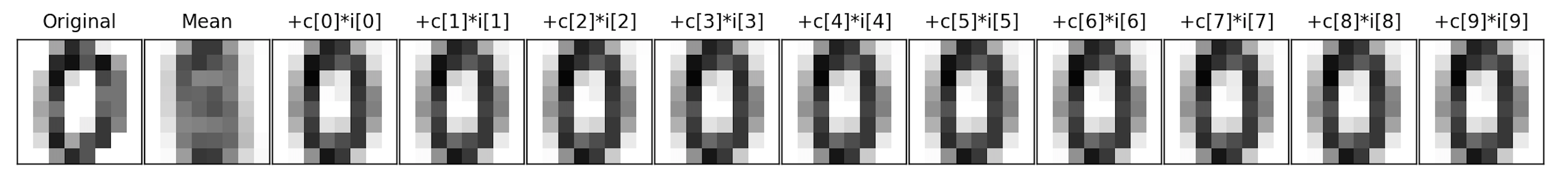
The next image is the overall mean, and each subsequent image is adding another component to the previous. For this particular scan, the mean plus its first component is enough to see that it's a 0.
For example, assuming the appropriate libraries are loaded:
from sklearn.decomposition import PCA
  pca = PCA()
  Xproj = pca.fit_transform(digits.data)
  showDigit(pca.mean_, f"Mean for digits")
  plt.imshow(pca.mean_.reshape(8,8),cmap='binary', interpolation='nearest',clim=(0, 16))
  plt.title("Mean for digits")
  plt.show()
  approxAnswer = approxDigits(8,Xproj[1068], pca.mean_, pca.components_)
  plt.imshow(approxAnswer.reshape(8,8),cmap='binary', interpolation='nearest',clim=(0, 16))
  plt.title("mean + 8 components for digits[1068]")
plt.show()digits[1068]:


Note: you should submit a file with only the standard comments at the top, this function, and any helper functions you have written. The grading scripts will then import the file for testing.
Classwork 10.1: Due 1:45pm, Wednesday, 1 November. The first part of the classwork focuses on principal components analysis (PCA) and is on paper. To receive credit, make sure to turn in your paper with your name and EmpID by the end of lecture.
Classwork 10.2: Due 3pm, Wednesday, 1 November. Available during Lecture 10 on Gradescope, this classwork focuses on distance metrics. To get the most out of this exercise, bring a device with you that can access Gradescope's online assignments.
Using Google Maps API, we generated the amount of time it would take to travel between the following landmarks:
- Bronx Zoo (Bronx),
- Empire State Building (Manhattan),
- National Lighthouse Museum (Staten Island),
- FDR Four Freedoms Park (Roosevelt Island),
- Citi Field (Queens),
- Coney Island (Brooklyn), and
- Hunter College (Manhattan)
Of the three, which best estimates the (aerial) distance?

Classwork 11.1: Due 1:45pm, Wednesday, 8 November. Available during Lecture 11 on Gradescope, this classwork builds intuition on clustering.
Classwork 11.2: Due 3pm, Wednesday, 8 November. In the second part of Lecture 11, we will start Program 5. Having successfully started the third program to Gradescope (i.e. a positive score) by the end of break gives credit for this classwork. You do not need to complete the thid program or submit anything extra, we will generate the scores directly by if you have submitted an attempt to Gradescope.
Classwork 12.1: Due 1:45pm, Wednesday, 15 November.
Write a program that asks the user for the name of an input HTML file and the name of an output CSV file. Your program should use regular expressions (see Chapter 12.4 for using the re package in Python) to find all links in the input file and store the link text and URL as columns: Title and URL in the CSV file specified by the user. For the URL, strip off the leading https:// or http:// and any trailing slashes (/):
For example, if the input file is:
<html>
<head><title>Simple HTML File</title></head>

<body>
  <p> Here's a link for <a href="http://www.hunter.cuny.edu/csci">Hunter CS Department</a>
  and for <a href="https://stjohn.github.io/teaching/data/fall21/index.html">CSci 39542</a>.  </p>

  <p> And for <a href="https://www.google.com/">google</a>
</body>
</html>
Enter input file name: simple.html
Enter output file name: links.csvlinks.csv would be:
Title,URL
Hunter CS Department,www.hunter.cuny.edu/csci
CSci 39542,stjohn.github.io/teaching/data/fall21/index.html
google,www.google.com
Note: you should submit a file with only the standard comments at the top that you attended lecture in the introductory comment (see Classwork 2 for details). The grading scripts will run your program directly on several different test cases, supplying the names of the files. If you do not ask for input in your program (e.g. ask for the input and output file names), the autograder will time-out waiting.
Classwork 12.2: Due 3pm, Wednesday, 15 November. Available during Lecture 12 on Gradescope, this classwork focuses on SQL. To get the most out of this exercise, bring a device with you that can access Gradescope's online assignments.
Classwork 13.1: Due 1:45pm, Wednesday, 29 November. Available during Lecture 13 on Gradescope, this classwork focuses on SQL. To get the most out of this exercise, bring a device with you that can access Gradescope's online assignments.
Classwork 13.2: Due 3pm, Wednesday, 29 November. In the second part of Lecture 13, we will start Program 6. Having successfully started the third program to Gradescope (i.e. a positive score) by the end of break gives credit for this classwork. You do not need to complete the thid program or submit anything extra, we will generate the scores directly by if you have submitted an attempt to Gradescope.
Midterm Exam
The midterm exam has two parts:
- Written Exam: will be Wednesday, 11 October, 11:30 am-12:45pm.
- Coding Exam: will be Wednesday, 11 October, 1:00-2:15pm.
For those who requested special accommodations:
- If you submitted a request for a borrowed laptop, your seat will be up front for both exams.
- For those requesting to take the exam at alternate times due to a documented learning disability or religious observance, we will reach out and coordinate a time to complete the exam early.
- Otherwise, your assigned seat is alphabetical by first name.
Written Examination
The written exam is on Wednesday, 11 October, 11:30am-12:45pm.Logistics:
- There is assigned seating (see above for details).
- To get credit for the exam, you must also turn in the signed attendance sheet before leaving.
Exam Rules:
- Leave your Hunter College ID on your desk to be checked during the exam.
- You may have one 8.5"x11" page of notes (content written on front and back).
- You may not seek outside help during the exam and no electronics are allowed including computers, phones, smart watches, etc.
Format and Preparing:
- The first pages of the exam include the first 4 pages of DS 100 Reference Sheet. Read over it as your design your single sheet of notes, since using the reference sheet could open up room for additional information on your notesheet.
- The written exam has 5 multiple-part questions on the material covered in lecture, classwork, and programming assignments, as well as the reading.
- The questions are similar to those given for past DS 100 exams. Their website contains the exams, as well as solutions. While we used their textbook, our course had slightly different focus (most notably, less statistics), as such not all problems are on their exams fit our course.
- Work through the past exams (with solutions) posted to the class Blackboard page.
Coding Examination
The coding exam is on Wednesday, 11 October, 1:00-2:15pm, in the style of the coding challenges during class.Logistics:
- The coding exam is administered on HackerRank, using Python 3.6+, libraries used in programming assignments and quizzes, and SQL.
- It is given in two 30-minute parts with a short break in between.
- There are multiple versions of the exam. To access your version, use the passwords on the attendance sheet at your assigned seat.
- To get credit for the exam, you must also turn in the signed attendance sheet before leaving.
Exam Rules:
- Leave your Hunter College ID on your desk to be checked during the exam.
- You may have one 8.5"x11" page of notes (content written on front and back).
- The exam must be taken on a laptop or tablet computer (no phones). You may use your own laptop or a department laptop (must be request in advance).
- You may not seek outside help during the exam, including leaving the window once you have started the exam.
Preparing: The exam covers the material covered in lecture, and classwork, and programming assignments, as well as the reading. To prepare:
- Bring the laptop (and its charging cables) you plan to use to the lecture on Wednesday, 4 October. Test that the power outlets work then, so, adjustments can be made before the exam.
- Work through the lecture coding challenges. Think about variations: what could we ask that's similar? These challenges make excellent exam questions.
Programming Assignments
Unless otherwise noted, programming assignments are submitted on the course's Gradescope site and are written in Python. The autograders expect a.py file and do not accept iPython notebooks.
Also, to receive full credit, the code should be compatible with Python 3.6 (the default for the Gradescope autograders) and written in good style.
Program 1: School Counts. Due noon, Friday, 8 September.
Program 2: School Success. Due noon, Friday, 22 September.
Program 3: Cookie Pricing. Due noon, Friday, 6 October.
Program 4: Taxi Classifiers. Due noon, Friday, 3 November.
Program 5: Neighborhood Clusters. Due noon, Friday, 17 November.
Program 6: Neighborhood Queries. Due noon, Friday, 8 December.
The grade for the project is a combination of grades earned on the milestones (e.g. deadlines during the semester to keep the projects on track) and the overall submitted program. If you choose not to complete the project, your final exam grade will replace its portion of the overall grade.
Learning Objective: to refresh students' knowledge of dictionaries and string functions of core Python, use constant models, and build competency with open source data portals.
Learning Objective: to build competency with Pandas for storing and cleaning data, use linear models, and introduce catergorical encoding.
Learning Objective: to build models with multiple linear regression and with polynomial features, use regularization techniques to better fit models, and use standard testing packages.
Learning Objective: to train and validate different models for classifying data.
Learning Objective: to enhance data cleaning skills and build understanding of clustering algorithms.
Learning Objective: To reinforce new regular expression and SQL skills to query and aggregate data.
Project
A final project is optional for this course.
Projects should synthesize the skills acquired in the course to analyze and visualize data on a topic of your choosing. It is your chance to demonstrate what you have learned, your creativity, and a project that you are passionate about. The intended audience for your project is your classmates as well as tech recruiters and potential employers.
Milestones
The project is broken down into smaller pieces that must be submitted by the deadlines below. For details of each milestone, see the links. The project is worth 25% of the final grade. The point breakdown is listed as well as the submission windows and deadlines. All components of the project are submitted via Gradescope unless other noted.
| Deadline: | Deliverables: | Points: | Submission Window Opens: |
|---|---|---|---|
| Tue, October 10, 2023 | Opt-In | Wed, September 20, 2023 | |
| Fri, October 22, 2023 | Proposal | 50 | Thu, October 12, 2023 |
| Fri, November 10, 2023 | Project Draft/Interim Check-In | 25 | Sat, October 23, 2023 |
| Friday, December 2, 2023 | Final Project Code Submission | 100 | Sat, November 11, 2023 |
| Friday, December 2, 2023 | Final Project Demonstration - Slides | 10 | Sat, November 11, 2023 |
| Friday, December 2, 2023 | Final Project Demonstration - Live Demo or Video Recording | 10 | Sat, November 11, 2023 |
| Total Points: | 200 | ||
Project Opt-In
Review the following FAQs before filling out the Project Opt-In form (available on Gradescope on September 20).- Is the final project mandatory?
No, the final project is optional for this course. - Will the project be difficult?
Expect the project to be time consuming because we will hold you to a high standard. However, in turn, we hope that this will produce a high quality project that you could proudly add to your coding portfolio, to showcase when seeking internships and full-time jobs. - What counts as "opting in" to the project?
That's easy. Your response to this Gradescope assignment counts as your "opt in". If you respond "No" or do not submit this assignment before the deadline due date, we will count you as having "opted out". - What happens after I "opt in"?
If you "opt in", we will continue to send you information on completing the next steps for the final project via Gradescope. If you "opt out", you will no longer receive follow up assignments for the project. - Does "opting in" place me under obligation to complete the project?
Yes and no. We would like you to seriously consider your availability before making this commitment. Likewise, we would like to focus our time to help those who are serious about doing this project. That being said, if you decide midway through the process that you no longer have the time nor capacity to complete the project, no harm no foul, your final written exam will once again be weighted 40% of your cumulative grade (see more in the question below). - How does the final project factor into my final grade?
If you choose to do the project, your final exam will be worth 25% of your overall course grade:- Optional Project: 25%
- Final Exam: 25%
- Final Exam: 50%
Project Proposal
The window for submitting proposals opens October 12. If you would like feedback and the opportunity to resubmit for a higher grade, submit early in the window. Feel free to re-submit as many times as you like, up until the assignment deadline. The instructing team will work hard to give feedback on your submission as quickly as possible, and we will grade them in the order they were received.
The proposal is split into the following sections:
- Overview:
Think of the overview section as the equivalent of an abstract in a research paper or an elevator pitch for the project. The following questions will help you frame your thoughts if you ever have to succinctly describe your project in an interview:- Title: should capture the topic/theme of your project.
- Objective: In 1 to 2 sentences, succinctly describe what you are hoping to accomplish in this project in simple, non technical English.
- Importance: In 1 to 2 sentences, describe why this project has personal significance to you.
- Originality: In 1 to 2 sentences, describe why you believe this project idea is unique and original.
- Background Research:
In this section, please prove to us that you have already done research in the project you are proposing by answering the questions below.- Key Term Definitions: What are some terms specific to your project that someone else might not know? List and define these terms here.
- Existing Solutions: What are some existing solutions (if any) that are already available for your problem. What are the drawbacks to these solutions?
- Data:
In order to write a successful proposal, you must already have obtained the data and done basic exploratory analysis on it, enough so that you feel confident you have enough data to answer the questions you wish to explore. We cannot stress this enough: You must use NYC specific data that is publicly available. If your data does not fit this criteria, your proposal will be rejected.The following questions will guide you through some criteria you should be using to assess if the data you have is enough for a successful project.
- Data Source: Include a list of your planned data source(s), complete with URL(s) for downloading. All data must be NYC specific and must be publicly available.
- Data Volume: How many columns in your dataset? How many rows? If you are joining multiple datasets together, please tell us how many rows and columns remain after the data has been merged into a single dataset.
- Data Richness: What type of data is in your dataset? You don't need to describe every column. A generalized overview is fine. (e.g. "My data contains 311 complaint types, the date the complaints are created and closed, as well as a description of the complaint"). If you found a data dictionary, feel free to link us to that as well.
- The Predictive Model:
A strong data science project should demonstrate your knowledge of predictive modeling. We will be covering models extensively in the latter half of the course. At this stage of the proposal writing, we will not have covered all the modeling techniques yet, so it's okay to be a bit vague here.Hint: Look ahead in the textbook at the chapters on "Linear Modeling" and "Multiple Linear Modeling" for the running examples of models.
- The Predicted (Y): Which column in the dataset are you interested in predicting?
- The Predictors (X's): Which column(s) in the dataset will be used to predict the column listed above?
- Python Dependencies: What Python libraries and dependencies will you be using?
- Security and Privacy Considerations: Will you be working with personal identifiable information (PII)? Can your model be mis-used for evil, not good? If so, how do you plan to mitigate that?
- The Visualization:
A key part of making a great data science portfolio are the visualizations. This is a quick and elegant way of showcasing your work during the job hunting process, even to a non-technical audience.Thus, a major part of this final project will center around making the following three types of visualizations with the data you choose. If your data cannot support all three types of visualizations, then please, reconsider choosing another dataset.
- Summary Statistics Plots: Write out in detail at least 3 types of summary statistics graphs you plan to make with your data (e.g. "I plan to make a histogram using the column X").
- Map Graphs: Write out in detail how you plan to make at least 1 map data visualization using your data (e.g. "I plan to create a choropleth map to visualize the volume of 311 service requests in NYC in 2021").
- Model Performance Plots: At the time of writing this proposal, we would not have covered how to visualize model accuracy yet. So, no worries if this part is still confusing to you. Give it your best shot on explaining what kind of visualization you think will best showcase that your model is "successful" and "accurate".
Project Interim Check-In
The interim check-in is submitted via Gradescope and contains:
- Title and Major Changes:
- Title: should capture the topic/theme of your project.
- Major Changes: Has there been any changes to the focus of your project since the project proposal? If none, write "None".
If there has been changes, explain why (e.g. found more data to enrich my dataset than what was originally described in the proposal).
- Summary Statistics:
- Upload the Visualization: Upload at least one summary statistics plot you've made so far. (File format accepted: PNG, JPEG, JPG)
- Inference Based on the Visualization: In your own words, what can you infer from this graph?
- Map Graphs:
- Upload the Visualization: Upload at least one map graph you've made so far. (File format accepted: PNG, JPEG, JPG)
- Inference Based on the Visualization: In your own words, what can you infer from this graph?
- Model Performance Plots:
- Upload the Visualization: Upload at least one model accuracy plot you've made so far. (File format accepted: PNG, JPEG, JPG)
- Inference Based on the Visualization: In your own words, what can you infer from this graph?
Final Project & Website Submission
Submission Instructions:
- Submit on Gradescope under "3. Final Project & Website Submission".
- Submit your code as one single Python .py file.
- Submit the URL of the website in the introductory comment section of the Python file, preceded by "URL:" so that it can be picked up by the Autograder.
- Submit the code you wrote for your project in the body of the Python file.
For example, for the student, Thomas Hunter, the opening comment of his project might be:
"""
Name:       Thomas Hunter
Email:      thomas.hunter1870@hunter.cuny.edu
Resources:  Used python.org as a reminder of Python 3 print statements.
Title:      My project
URL:        https://www.myproject.com
"""
The Gradescope Autograder will check for the Python file and that includes the title, the resources, and the URL of your website. After the submission deadline, the code and the website will be graded manually for code quality and data science inference.
For manual grading of the project, we are grading for the following:
- Overall Code Quality (code):
We are looking for production level code. No stream of consciousness scripting please. Everything should be in functions, cleanly formatted, and optimized for performance.
- Good Use of the Data (code & website):
We are looking for evidence that you did analysis on a non-trivial sized dataset and used the data in a meaningful way, drawing from the data cleaning, inference, visualization, and predictive modeling techniques you've learned this semester. Please use the questions in the project proposal and the interim check-in as guidelines for what we are expecting from you.
- Model Inference (code & website):
We covered a number of predictive modeling techniques in this course, from regularization to linear regression to classification to to SVMs to more. In both the proposal and the interim check in, we have asked you to brainstorm and show us some interim output on the predictive model(s) you have used on your data. Now for the final submission, we ask that you show us 1) the code and output for the final model you chose and 2) the reasoning behind why you chose this model and finally, 3) any inference, interpretation, and insights from the final model results.
- High Quality Data Visualizations (code & website):
Just like the project interim check-in. We would like to see three types of visualizations: 1) at least one exploratory data analysis graph 2) at least one map related graph and 3) at least one model inference graph. All graphs must be made by you, in Python. Please also make the code available in the Python file submission. If you've already made the visualizations during the interim check-in, we hope that you would take the time to clean them up so that they could be a great show-case of your data visualization skills on your website.
Project Demonstration
For the last part of the project, we would like to you to prepare a lightning demo. This composes of two parts:
- Two slides that serve as a graphical overview ("lightning talk" slides) of your project.
- To be submitted under "4. Final Project Demonstration - Slides"
- Slide 1: the front image and title from website, as well as your name
- Slide 2: discoveries & conclusions (with images)
- It's completely acceptable to re-use what you wrote on the website and the data visualizations you've submitted for "Final Project & Website Submission" here.
- An in-person 30 second demo of your project OR a pre-recorded 30 second video demo.
- Grading rubric is the same whether you choose in-person or pre-recorded. More details under "5. Final Project Demonstration - Video Recording".
- If you choose to do this in person, please note you will be expected present in class, in-person, on May 10th, after the coding exam.
- If you choose to do this via pre-recorded video recording, the video submission should be uploaded under "5. Final Project Demonstration - Video Recording". Please go to Gradescope to see see more instructions there.