Program 2: School Success
CSci 39542: Introduction to Data Science
Department of Computer Science
Hunter College, City University of New York
Spring 2023
Classwork Quizzes Homework Project
Program Description
Program 2: School Success. Due noon, Friday, 22 September.
Learning Objective: to build competency with Pandas for storing and cleaning data, use linear models, and introduce catergorical encoding.
Available Libraries: Core Python 3.6+, Pandas.
Data Sources: NYC Open Data: 2021 DOE High School Directory,
2020 DOE High School Directory,
2019 DOE High School Directory.
Sample Datasets: 2021_DOE_High_School_Directory_SI.csv (2021 dataset restricted to Staten Island schools) and
2020_DOE_High_School_Directory_late_start.csv (schools with 9am start times in 2020 dataset).
The second program uses the same DOE school directory datasets as Program 1. Instead of using string and file I/O from core Python, this program uses Pandas to store and manipulate the data. The linear models built in this program are more complex than the simple constant models from the first program. This program follows a similar structure:
- focuses on a data set, usually related to NYC,
- cleans the data to be used for analysis,
- builds a model, using some of the data,
- evaluates how well the model at predicting, using the rest of the data, and
- incorporates tests that the writen code perform correctly.
Programs are submitted via Gradescope (see general notes above for details) and can only use the libraries specified above (echoing the restrictions of technical screenings).

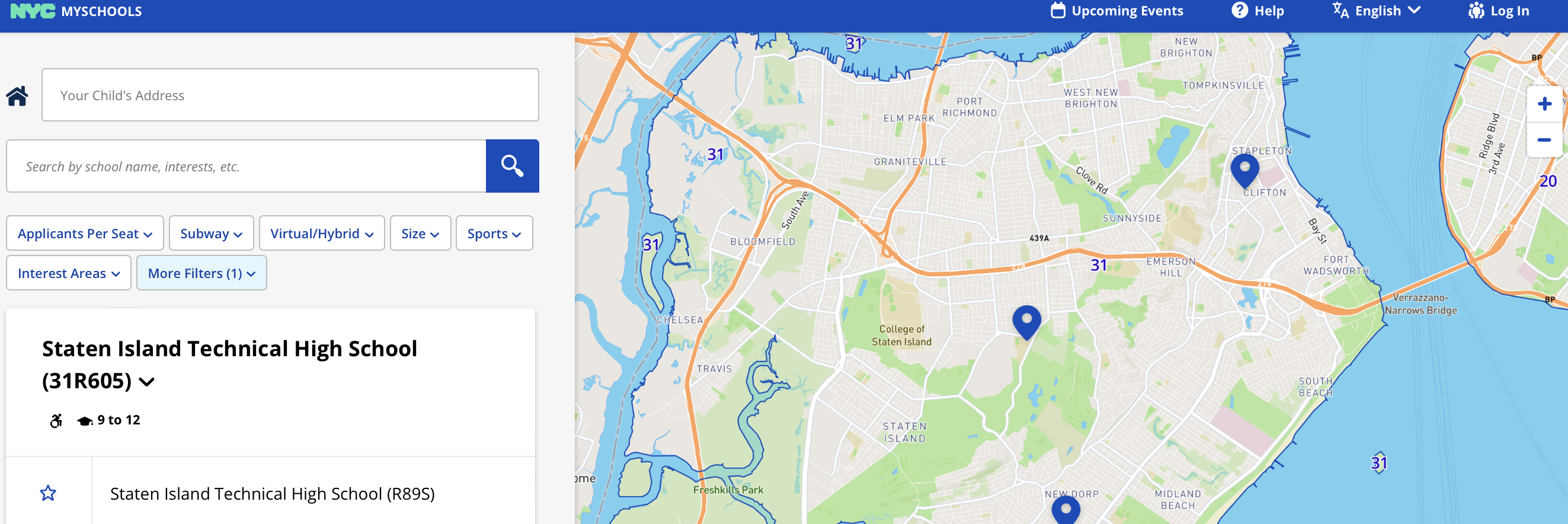
NYC OpenData
Much of the data collected by New York City agencies is publicly available at NYC Open Data. For this program, we will use the overview of high schools maintained by the Department of Education and available each year for rising 9th graders to choose a high school:
See Program 1 for the steps needed to download the datasets for testing.
The datasets have a large number (448!) columns:
dbn,school_name,borocode,url,overview_paragraph,diversity_in_admissions,diadetails,school_10th_seats,academicopportunities1,academicopportunities2,academicopportunities3,academicopportunities4,academicopportunities5,academicopportunities6,ell_programs,language_classes,advancedplacement_courses,diplomaendorsements,neighborhood,shared_space,campus_name,building_code,location,phone_number,fax_number,school_email,website,recruitment_website,sqr_website,subway,bus,gradespan,finalgrades,total_students,freshmanschedule,start_time,end_time,addtl_info1,extracurricular_activities,psal_sports_boys,psal_sports_girls,psal_sports_coed,school_sports,graduation_rate,pct_stu_safe,attendance_rate,pct_stu_enough_variety,college_career_rate,girls,boys,pbat,international,specialized,transfer,ptech,earlycollege,school_accessibility_description,program1,program2,program3,program4,program5,program6,program7,program8,program9,program10,program11,program12,interest1,interest2,interest3,interest4,interest5,interest6,interest7,interest8,interest9,interest10,interest11,interest12,prgdesc1,prgdesc2,prgdesc3,prgdesc4,prgdesc5,prgdesc6,prgdesc7,prgdesc8,prgdesc9,prgdesc10,prgdesc11,prgdesc12,common_audition1,common_audition2,common_audition3,common_audition4,common_audition5,common_audition6,common_audition7,common_audition8,common_audition9,common_audition10,common_audition11,common_audition12,auditioninformation1,auditioninformation2,auditioninformation3,auditioninformation4,auditioninformation5,auditioninformation6,auditioninformation7,auditioninformation8,auditioninformation9,auditioninformation10,auditioninformation11,auditioninformation12,seats9ge1,seats9ge2,seats9ge3,seats9ge4,seats9ge5,seats9ge6,seats9ge7,seats9ge8,seats9ge9,seats9ge10,seats9ge11,seats9ge12,grade9geapplicants1,grade9geapplicantsperseat1,grade9geapplicants2,grade9geapplicantsperseat2,grade9geapplicants3,grade9geapplicantsperseat3,grade9geapplicants4,grade9geapplicantsperseat4,grade9geapplicants5,grade9geapplicantsperseat5,grade9geapplicants6,grade9geapplicantsperseat6,grade9geapplicants7,grade9geapplicantsperseat7,grade9geapplicants8,grade9geapplicantsperseat8,grade9geapplicants9,grade9geapplicantsperseat9,grade9geapplicants10,grade9geapplicantsperseat10,grade9geapplicants11,grade9geapplicantsperseat11,grade9geapplicants12,grade9geapplicantsperseat12,grade9gefilledflag1,grade9gefilledflag2,grade9gefilledflag3,grade9gefilledflag4,grade9gefilledflag5,grade9gefilledflag6,grade9gefilledflag7,grade9gefilledflag8,grade9gefilledflag9,grade9gefilledflag10,grade9gefilledflag11,grade9gefilledflag12,seats9swd1,seats9swd2,seats9swd3,seats9swd4,seats9swd5,seats9swd6,seats9swd7,seats9swd8,seats9swd9,seats9swd10,seats9swd11,seats9swd12,grade9swdapplicants1,grade9swdapplicantsperseat1,grade9swdapplicants2,grade9swdapplicantsperseat2,grade9swdapplicants3,grade9swdapplicantsperseat3,grade9swdapplicants4,grade9swdapplicantsperseat4,grade9swdapplicants5,grade9swdapplicantsperseat5,grade9swdapplicants6,grade9swdapplicantsperseat6,grade9swdapplicants7,grade9swdapplicantsperseat7,grade9swdapplicants8,grade9swdapplicantsperseat8,grade9swdapplicants9,grade9swdapplicantsperseat9,grade9swdapplicants10,grade9swdapplicantsperseat10,grade9swdapplicants11,grade9swdapplicantsperseat11,grade9swdapplicants12,grade9swdapplicantsperseat12,grade9swdfilledflag1,grade9swdfilledflag2,grade9swdfilledflag3,grade9swdfilledflag4,grade9swdfilledflag5,grade9swdfilledflag6,grade9swdfilledflag7,grade9swdfilledflag8,grade9swdfilledflag9,grade9swdfilledflag10,grade9swdfilledflag11,grade9swdfilledflag12,seats1specialized,seats2specialized,seats3specialized,seats4specialized,seats5specialized,seats6specialized,applicants1specialized,applicants2specialized,applicants3specialized,applicants4specialized,applicants5specialized,applicants6specialized,appperseat1specialized,appperseat2specialized,appperseat3specialized,appperseat4specialized,appperseat5specialized,appperseat6specialized,seats101,seats102,seats103,seats104,seats105,seats106,seats107,seats108,seats109,seats1010,seats1011,seats1012,eligibility1,eligibility2,eligibility3,eligibility4,eligibility5,eligibility6,eligibility7,eligibility8,eligibility9,eligibility10,eligibility11,eligibility12,admissionspriority11,admissionspriority21,admissionspriority31,admissionspriority41,admissionspriority12,admissionspriority22,admissionspriority32,admissionspriority42,admissionspriority13,admissionspriority23,admissionspriority33,admissionspriority43,admissionspriority14,admissionspriority24,admissionspriority34,admissionspriority44,admissionspriority15,admissionspriority25,admissionspriority35,admissionspriority45,admissionspriority16,admissionspriority26,admissionspriority36,admissionspriority46,admissionspriority17,admissionspriority27,admissionspriority37,admissionspriority47,admissionspriority18,admissionspriority28,admissionspriority38,admissionspriority48,admissionspriority19,admissionspriority29,admissionspriority39,admissionspriority49,admissionspriority110,admissionspriority210,admissionspriority310,admissionspriority410,admissionspriority111,admissionspriority211,admissionspriority311,admissionspriority411,admissionspriority112,admissionspriority212,admissionspriority312,admissionspriority412,offer_rate1_1,offer_rate2_1,offer_rate3_1,offer_rate4_1,offer_rate1_2,offer_rate2_2,offer_rate3_2,offer_rate4_2,offer_rate1_3,offer_rate2_3,offer_rate3_3,offer_rate4_3,offer_rate1_4,offer_rate2_4,offer_rate3_4,offer_rate4_4,offer_rate1_5,offer_rate2_5,offer_rate3_5,offer_rate4_5,offer_rate1_6,offer_rate2_6,offer_rate3_6,offer_rate4_6,offer_rate1_7,offer_rate2_7,offer_rate3_7,offer_rate4_7,offer_rate1_8,offer_rate2_8,offer_rate3_8,offer_rate4_8,offer_rate1_9,offer_rate2_9,offer_rate3_9,offer_rate4_9,offer_rate1_10,offer_rate2_10,offer_rate3_10,offer_rate4_10,offer_rate1_11,offer_rate2_11,offer_rate3_11,offer_rate4_11,offer_rate1_12,offer_rate2_12,offer_rate3_12,offer_rate4_12,requirement_1_1,requirement_2_1,requirement_3_1,requirement_4_1,requirement_5_1,requirement_1_2,requirement_2_2,requirement_3_2,requirement_4_2,requirement_5_2,requirement_1_3,requirement_2_3,requirement_3_3,requirement_4_3,requirement_5_3,requirement_1_4,requirement_2_4,requirement_3_4,requirement_4_4,requirement_5_4,requirement_1_5,requirement_2_5,requirement_3_5,requirement_4_5,requirement_5_5,requirement_1_6,requirement_2_6,requirement_3_6,requirement_4_6,requirement_5_6,requirement_1_7,requirement_2_7,requirement_3_7,requirement_4_7,requirement_5_7,requirement_1_8,requirement_2_8,requirement_3_8,requirement_4_8,requirement_5_8,requirement_1_9,requirement_2_9,requirement_3_9,requirement_4_9,requirement_5_9,requirement_1_10,requirement_2_10,requirement_3_10,requirement_4_10,requirement_5_10,requirement_1_11,requirement_2_11,requirement_3_11,requirement_4_11,requirement_5_11,requirement_1_12,requirement_2_12,requirement_3_12,requirement_4_12,requirement_5_12,code1,method1,code2,method2,code3,method3,code4,method4,code5,method5,code6,method6,code7,method7,code8,method8,code9,method9,code10,method10,code11,method11,code12,method12,primary_address_line_1,city,postcode,state_code,Borough,Latitude,Longitude,Community Board,Council District,Census Tract,BIN,BBL,NTA
For this assignment, we are going to focus on a subset of these columns, listed below.
Cleaning Data
Note: for this assignment, we are using native Python libraries and the data cleaning library Pandas. See Lectures 2 and 3 and the Resources page for more details on using Pandas.
Make sure you have downloaded some test data sets to your device. Start a .py file that contains your introductory comment (see General Notes above for format). The next step is to format the data for analysis. Add the following to your file, testing as you go:
-
import_data(file_name):This function takes as one input parameter:-
file_name: the name of a CSV file containing 2021 DOE High School Directory from OpenData NYC.
- only the columns, in the order below:
are kept (e.g. all others dropped).dbn,school_name,NTA,graduation_rate,pct_stu_safe,attendance_rate,college_career_rate,language_classes,advancedplacement_courses,method1,overview_paragraph - Any rows with missing values for
graduation rateare dropped.
-
-
impute_numeric_cols(df):This function takes one input:-
df: a DataFrame containing DOE High School from OpenData NYC.
['pct_stu_safe','attendance_rate', 'college_career_rate']are replaced with the median of the respective column.
Returns the resulting DataFrame. -
-
compute_count_col(df,col):This function takes two inputs:-
df: a DataFrame containing DOE High School from OpenData NYC. -
col: a column name indfthat contains a list of items separated by commas.
df[col].
Returns the resulting Series. -
-
encode_categorical_col(col):This function takes one input parameter:-
col: a column of categorical data.
Mandarin, French, Arabic, Spanish, then the resulting columns would be labeled with those languages and sorted:Arabic, French, Mandarin, Spanish.
Note: we presented several different ways to categorically encode nomial data in Lecture 3. While the book details an approach Chapter 15, it uses scikit-learn (sklearn) which is not included in this program. You may find Panda's Series.str.get_dummies useful. -
-
split_test_train(df, xes_col_names, y_col_name,
        frac=0.25, random_state=922):
This function takes 5 input parameters:-
df: a DataFrame -
y_col_name: the name of the column of the dependent variable. -
xes_col_names: a list of columns that contain the independent variables. -
frac: accepts a float between 0 and 1 and represents the proportion of the data set to use for training. This parameter has a default value of 0.25. -
random_state: Used as a seed to the randomization. This parameter has a default value of 922.
- Create a new DataFrame,
df_testusing panda's sample function to create a test set withfracof the rows andrandom_statefor the random seed. - Makes a copy of the DataFrame,
dfand call itdf_train. - Drop the rows in
df_testfromdf_train(e.g.df_train = df_train.drop(df_test.index)) - Return
df_train[xes_col_names],df_test[xes_col_names],df_train[y_col_name],df_test[y_col_name].
-
For example, starting with the Staten Island data set:
file_name = 'fall23/program02/2021_DOE_High_School_Directory_SI.csv'
df = import_data(file_name)
print(f'There are {len(df.columns)} columns:')
print(df.columns)
print('The dataframe is:')
print(df)There are 11 columns:
Index(['dbn', 'school_name', 'NTA', 'graduation_rate', 'pct_stu_safe',
'attendance_rate', 'college_career_rate', 'language_classes',
'advancedplacement_courses', 'method1', 'overview_paragraph'],
dtype='object')
The dataframe is:
dbn school_name ... method1 overview_paragraph
1 31R047 CSI High School for International Studies ... Open Our challenging and academically demanding pro...
2 31R064 Gaynor McCown Expeditionary Learning School ... Ed. Opt. McCown is a college preparatory school partner...
3 31R080 Michael J. Petrides School, The ... Ed. Opt. Petrides is a comprehensive college preparator...
4 31R440 New Dorp High School ... Ed. Opt. New Dorp High School is a comprehensive high s...
5 31R445 Port Richmond High School ... Screened Port Richmond High School is a comprehensive C...
6 31R450 Curtis High School ... Open Curtis High School is a Community School whose...
7 31R455 Tottenville High School ... Ed. Opt. Tottenville High School has long been recogniz...
8 31R460 Susan E. Wagner High School ... Screened Susan E. Wagner High School consists of 16 uni...
9 31R600 Ralph R. McKee Career and Technical Education ... ... Ed. Opt. McKee prepares you for college, career, and li...
10 31R605 Staten Island Technical High School ... Test SI Technical High School provides a robust lib...
[10 rows x 11 columns]Note that there are 11 high schools in Staten Island, but one (Eagle Academy) was new and didn't have a graduation rate, so, was dropped.
Looking at the schools who start after 9am:
file_name = 'fall23/program02/2020_DOE_High_School_Directory_late_start.csv'
df_late = import_data(file_name)
print('The numerical columns are:')
print(df_late[ ['dbn','pct_stu_safe','attendance_rate','college_career_rate'] ])
The numerical columns are:
       dbn  pct_stu_safe  attendance_rate  college_career_rate
0   01M696          0.92             0.95                 0.92
1   07X334          0.89             0.90                 0.35
2   02M543          0.92             0.84                 0.75
3   14K685          0.94             0.83                 0.42
4   02M546          0.80             0.90                 0.78
5   02M376          0.97             0.93                 0.79
6   19K404          0.87             0.86                 0.74
7   20K490          0.80             0.90                 0.57
9   27Q334          0.92             0.83                  NaN
10  30Q301          0.94             0.93                 0.84
11  28Q328          0.87             0.87                 0.88
12  14K561          0.94             0.89                 0.76
13  31R450          0.76             0.85                 0.60
14  02M298          0.89             0.87                 0.65
15  04M555          0.97             0.95                 0.95
16  10X353          0.95             0.88                 0.69
17  02M420          0.90             0.91                 0.73
18  10X351          0.83             0.76                 0.39
19  20K445          0.75             0.86                 0.63
20  21K337          0.90             0.90                 0.46
21  18K633          0.92             0.89                 0.81
22  23K514          0.88             0.82                 0.37
23  02M294          0.89             0.87                 0.78
24  30Q575          0.86             0.93                 0.62
26  28Q440          0.77             0.90                 0.72
27  24Q299          0.97             0.98                 0.99
28  16K765          0.87             0.72                  NaN
29 09X403 0.89 0.83 0.47college_career_rate. We will fill those in (impute) with the median of the column:
df_late = impute_numeric_cols(df_late)
print(df_late[ ['dbn','pct_stu_safe','attendance_rate','college_career_rate'] ])
           dbn  pct_stu_safe  attendance_rate  college_career_rate
    0   01M696          0.92             0.95                0.920
    1   07X334          0.89             0.90                0.350
    2   02M543          0.92             0.84                0.750
    3   14K685          0.94             0.83                0.420
    4   02M546          0.80             0.90                0.780
    5   02M376          0.97             0.93                0.790
    6   19K404          0.87             0.86                0.740
    7   20K490          0.80             0.90                0.570
    9   27Q334          0.92             0.83                0.725
    10  30Q301          0.94             0.93                0.840
    11  28Q328          0.87             0.87                0.880
    12  14K561          0.94             0.89                0.760
    13  31R450          0.76             0.85                0.600
    14  02M298          0.89             0.87                0.650
    15  04M555          0.97             0.95                0.950
    16  10X353          0.95             0.88                0.690
    17  02M420          0.90             0.91                0.730
    18  10X351          0.83             0.76                0.390
    19  20K445          0.75             0.86                0.630
    20  21K337          0.90             0.90                0.460
    21  18K633          0.92             0.89                0.810
    22  23K514          0.88             0.82                0.370
    23  02M294          0.89             0.87                0.780
    24  30Q575          0.86             0.93                0.620
    26  28Q440          0.77             0.90                0.720
    27  24Q299          0.97             0.98                0.990
    28  16K765          0.87             0.72                0.725
    29  09X403          0.89             0.83                0.470
Using the compute_count_col twice, let's add in counts for languages & AP classes:
df_late['language_count'] = compute_count_col(df_late,'language_classes')
df_late['ap_count'] = compute_count_col(df_late,'advancedplacement_courses')
print('High schools that have 9am or later start:')
print(df_late[ ['dbn','language_count','language_classes','ap_count','advancedplacement_courses'] ])
High schools that have 9am or later start:
    dbn  language_count                                   language_classes  ap_count                          advancedplacement_courses
0   01M696               5            French, Greek, Latin, Mandarin, Spanish         0                                                NaN
1   07X334               1                                             French         0                                                NaN
2   02M543               1                                            Spanish         2  AP English Literature and Composition, AP Unit...
3   14K685               1                                            Spanish         0                                                NaN
4   02M546               1                                            Spanish         6  AP Biology, AP Calculus AB, AP Computer Scienc...
5   02M376               1                                            Spanish         4  AP Calculus AB, AP English Language and Compos...
6   19K404               1                                            Spanish         5  AP Biology, AP Computer Science A, AP English ...
7   20K490               6  Arabic, French, Greek, Italian, Mandarin, Spanish        20  AP 2-D Art and Design, AP Biology, AP Calculus...
9   27Q334               1                                            Spanish         6  AP Biology, AP Computer Science Principles, AP...
10  30Q301               1                                             French         6  AP Calculus AB, AP Computer Science Principles...
11  28Q328               2                                    French, Spanish         5  AP Biology, AP Calculus AB, AP Chemistry, AP C...
12  14K561               2                    American Sign Language, Spanish         7  AP Calculus AB, AP English Language and Compos...
13  31R450               3                           French, Italian, Spanish        10  AP Calculus AB, AP Computer Science Principles...
14  02M298               1                                            Spanish         5  AP Biology, AP Calculus AB, AP English Languag...
15  04M555               1                                            Spanish         7  AP Calculus AB, AP Computer Science Principles...
16  10X353               4                  French, German, Japanese, Spanish         6  AP English Language and Composition, AP Englis...
17  02M420               1                                            Spanish        12  AP Art History, AP Biology, AP Calculus AB, AP...
18  10X351               2                                  Japanese, Spanish         1                                         AP Seminar
19  20K445               4                 Arabic, Italian, Mandarin, Spanish        22  AP Biology, AP Calculus AB, AP Calculus BC, AP...
20  21K337               2                                  Mandarin, Spanish         0                                                NaN
21  18K633               1                                            Spanish         6  AP Biology, AP English Literature and Composit...
22  23K514               2                                    French, Spanish         4  AP Chemistry, AP English Language and Composit...
23  02M294               2                                    French, Spanish         0                                                NaN
24  30Q575               2                                    French, Spanish        10  AP Calculus AB, AP Calculus BC, AP English Lan...
26  28Q440               7  American Sign Language, French, Hebrew, Italia...        19  AP Art History, AP Biology, AP Calculus AB, AP...
27  24Q299               3                           Latin, Mandarin, Spanish         0                                                NaN
28  16K765               1                                            Spanish         3  AP Biology, AP English Literature and Composit...
29  09X403               2                                    French, Spanish         3  AP Calculus AB, AP French Language and Culture...
Continuing our example, we can add columns for the languages available, using one hot encoding:
df_langs = encode_categorical_col(df_late['language_classes'])
print(df_late['language_classes'].head(5))
print(df_langs.head(5))
print('Number of schools for each language:')
print(df_langs.sum(axis=0))
0    French, Greek, Latin, Mandarin, Spanish
1                                     French
2                                    Spanish
3                                    Spanish
4                                    Spanish
Name: language_classes, dtype: object

   American Sign Language  Arabic  French  German  Greek  Hebrew  Italian  Japanese  Latin  Mandarin  Spanish
0                       0       0       1       0      1       0        0         0      1         1        1
1                       0       0       1       0      0       0        0         0      0         0        0
2                       0       0       0       0      0       0        0         0      0         0        1
3                       0       0       0       0      0       0        0         0      0         0        1
4                       0       0       0       0      0       0        0         0      0         0        1

Number of schools for each language:
American Sign Language     2
Arabic                     2
French                    12
German                     1
Greek                      2
Hebrew                     1
Italian                    4
Japanese                   3
Latin                      2
Mandarin                   6
Spanish                   28
dtype: int64
To validate our models, we will randomly split the dataset into training and testing sets:
xes_cols = ['language_count','ap_count','pct_stu_safe','attendance_rate','college_career_rate']
y_col = 'graduation_rate'
x_train, x_test, y_train, y_test = split_test_train(df_late,xes_cols,y_col)
print(f'The sizes of the sets are:')
print(f'x_train has {len(x_train)} rows.\tx_test has {len(x_test)} rows.')
print(f'y_train has {len(y_train)} rows.\ty_test has {len(y_test)} rows.')
x_train has 22 rows.    x_test has 8 rows.
y_train has 22 rows.    y_test has 8 rows.
Once you have written your function, test it locally on the small test files. When it works, upload to Gradescope. Given the size of the files that we evaluate your code, you will find it much faster to develop and test the code in your IDE than debugging and testing in Gradescope.
Linear Regression Model
Last program, we built constant models which predicts the same (constant) values for all inputs. For this program, we are building models that vary their output, based on the input. Our first models will be linear regression models where we find the line that best fits (using least square) the data. Chapter 15 sets a good foundation for this and includes many examples.
We will first implement the linear regression for a single independent (explanatory) variable and a dependent (outcome) variable using only Pandas (our next assigment we will use build more complex models and use packages that have implemented them).
-
compute_lin_reg(xes, yes): This function takes two inputs:xes: an iterables of numeric values representing the independent variableyes: an iterables of numeric values representing the dependent variable
- Compute the standard deviation of the
xesandyes. Call thesesd_xandsd_y. - Compute the correlation,
r, of thexesandyes. - Compute the slope,
theta_1, astheta_1 = r*sd_y/sd_x. - Compute the y-intercept,
theta_0, astheta_0 = average(yes) - theta_1 * average(xes) - Return
theta_0andtheta_1.
Continuing our example for the late start high schools:
coeff = {}
for col in xes_cols:
    coeff[col] = compute_lin_reg(x_train[col],y_train)
    print(f'for {col}, theta_0 = {coeff[col][0]} and theta_1 = {coeff[col][1]}')
for language_count, theta_0 = 0.8480569704034503 and theta_1 = 0.008590562417322539
for ap_count, theta_0 = 0.8461003017752102 and theta_1 = 0.0036611430972476005
for pct_stu_safe, theta_0 = 0.3139020169251634 and theta_1 = 0.6179008519044576
for attendance_rate, theta_0 = 0.05301553094638145 and theta_1 = 0.937016067877174
for college_career_rate, theta_0 = 0.5128147415423354 and theta_1 = 0.5026459501657516
Evaluating Our Models
The next part of program evaluates how well our linear models do at prediction. We will use a loss function, mean squared error and rooted mean squared error, introduced in Lecture 1 and Section 4.2.
-
predict(xes, theta_0, theta_1): This function takes three inputs:xes: an iterables of numeric values representing the independent variabletheta_0: the y-intercept of the linear regression modeltheta_1: the slope of the linear regression model
xes, under the linear regression model with y-intercepttheta_0and slopetheta_1. -
mse_loss(y_actual,y_estimate):This function takes two inputs:-
y_actual: a Series containing numeric values. -
y_estimate: a Series containing numeric values.
y_actualandy_estimate(e.g. the mean of the squares of the differences).
Note: a variation of this function was part of an earlier homework (Program 1) as well as in the textbook (using numpy). This is slightly different from both, as it takes lists (instead of dictionaries) and does not use the numpy library. It is included here to be used as a default argument for the error computation function below. -
-
rmse_loss(y_actual,y_estimate):This function takes two inputs:-
y_actual: a Series containing numeric values. -
y_estimate: a Series containing numeric values.
y_actualandy_estimate(e.g. the square root of the mean of the squares of the differences). -
-
compute_error(y_actual,y_estimate,loss_fnc=mse_loss): This function takes three inputs:-
y_actual: a Series containing numeric values. -
y_estimate: a Series containing numeric values. -
loss_fnc: function that takes two numeric series as input parameters and returns a numeric value. It has a default value of mse_loss.
loss_fncon the inputsy_actualandy_estimateis returned. -
Continuing our example of number of sentences in an overview:
coeff = {}
for col in xes_cols:
    coe = compute_lin_reg(x_train[col],y_train)
    coeff[col] = coe
print(f'for {col}, theta_0 = {coe[0]} and theta_1 = {coe[1]}')for language_count, theta_0 = 0.821969696969697 and theta_1 = 0.008721590909090911
for ap_count, theta_0 = 0.829236532747707 and theta_1 = 0.0021805968221160063
for pct_stu_safe, theta_0 = 0.3259265268281375 and theta_1 = 0.5869741569127364
for attendance_rate, theta_0 = -0.4082696527688132 and theta_1 = 1.4385568607202786
for college_career_rate, theta_0 = 0.4664578537197913 and theta_1 = 0.5575944180964911Lets see which explanatory variable did best on the testing data:
predicts = {}
errors = {}
min_error = 1
best = ""
for col in xes_cols:
    predicts[col] = predict(x_test[col], coe[0], coe[1])
    errors[col] = compute_error(y_test,predicts[col])
    print(f'Error on test data for {col} is {errors[col]}.')
    if errors[col] < min_error:
        min_error = errors[col]
        best = col

print(f'Column {col} has lowest error ({min_error}).')Error on test data for language_count is 1.4074577840833737.
Error on test data for ap_count is 21.589341577894185.
Error on test data for pct_stu_safe is 0.014732620032972344.
Error on test data for attendance_rate is 0.015958758340922953.
Error on test data for college_career_rate is 0.0016245415203027973.
Column college_career_rate has lowest error (0.0016245415203027973).The smallest losses are for college_career_rate, so, let's graph that to visualize the difference between the actual and predicted data. We first build a helper function to use for graphing.
import matplotlib.pyplot as plt
import seaborn as sns
def graph_data(df, col, coeff):
    """
    Function to graph the models
    """
    plt.scatter(df[col],df['graduation_rate'],label='Actual')
    predict_grad = predict(df_late[col],coeff[col][0],coeff[col][1])
    plt.scatter(df[col], predict_grad,label='Predicted')
    plt.title(f'{col} vs graduation_rate')
    plt.xlabel('graduation_rate')
    plt.ylabel(f'{col}')
    plt.legend()
    plt.show()

graph_data(df_late, 'college_career_rate',coeff)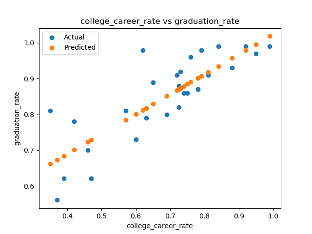
Testing Code
Each programming assignment includes functions that test that your code works (a "test suite"). We will first build these in core Python, and in future assignments (Programs 3-6), will introduce standard testing packages.
Your program should include the functions below that test if your functions above perform correctly. Each of these functions takes a function as an argument. You can write them in any order, but we have placed them easiest to hardest below:
-
test_compute_count_col(compute_fnc=compute_count_col): This test function takes one input:-
compute_fnc: a function that takes two input parameters (a DataFrame and the name of a categorical column) and returns a Series. It has a default value ofcompute_count_col.
compute_fncreturningTrueif thecompute_fncperforms correctly (e.g. computes the the count column) andFalseotherwise.Hint: we will test your function with three different functions: the correct one, one that returns the column, and one that always returns a DataFrame with the 3 specified columns having the same entry (42) for all rows.
-
-
test_predict(predict_fnc=predict): This test function takes one input:-
predict_fnc: a function that takes three input parameters (a Series and two numerics) and returns a Series. It has a default value ofpredict.
predict_fncreturningTrueif thepredict_fncperforms correctly (e.g. predicts the correct values) andFalseotherwise.Hint: we will test your function with three different functions: the correct one, one that returns the Series unchanged, and one that always returns a Series with the same entry (42) for all rows.
-
-
test_mse_loss(loss_fnc=mse_loss): This test function takes one input:-
loss_fnc: a function that takes three input parameter (two Series) and returns a numeric. It has a default value ofmse_loss.
loss_fncreturningTrueif theloss_fncperforms correctly (e.g. compute MSA) andFalseotherwise.Hint: we will test your function with three different functions: the correct one, one that always uses mean absolute error as its loss function, and one that always returns 42.
-
Trying first on the correct function:
print(f'test_compute_count_col(compute_count_col) returns {test_compute_count_col(compute_count_col)}.')test_compute_count_col(compute_count_col) returns True.Continuing our example with a function that returns the input columns values (instead of counts):
def same(df,col):
    return df[col]
print(f'test_compute_count_col(same) returns {test_compute_count_col(same)}.')test_compute_count_col(same) returns False.Notes
- You should submit a file with only the standard comments at the top, the specified functions, and any helper functions you have written. The grading scripts will then import the file for testing.
- If your file includes code outside of functions, either comment the code out before submitting or use a main function that is conditionally executed (see Think CS: Section 6.8 for details).