Program 5, CSci 39542: Data Science, Hunter College

Program 5: EMS Clusters
CSci 39542: Introduction to Data Science
Department of Computer Science
Hunter College, City University of New York
Fall 2023

Program Description

Program 5: EMS Clusters. Due noon, Friday, 17 November.
Learning Objective: to enhance data cleaning skills and build understanding of clustering algorithms.
Available Libraries: pandas, datetime, sklearn, and core Python 3.6+.
Data Sources:
Data Sources: 911 System Calls (NYC OpenData)
Sample Datasets:

Small dataset (1 day of calls for 1 borough): NYPD_Calls_Manhattan_4Jul2021.csv,
Midnight calls in January 2021 (all boroughs): NYPD_Calls_midnight_Jan2021.csv,
Larger dataset (1 month of calls for Queens): NYPD_Calls_Queens_Jan2021.csv

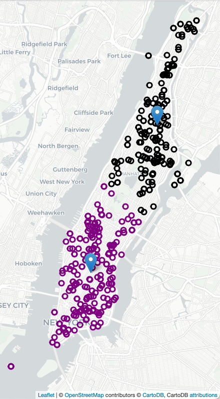
For this program, we are building on the clustering techniques from Lecture 11 and Classwork 11.1 which focused on different clustering algorithms. Decreasing ambulance response times improves outcomes and strategic placement of ambulance stations and overall allocation has been shown an effective approach. For example, here are all the calls for ambulances on 4 July 2021 in Manhattan (using Folium/Leaflet to create an interactive map):

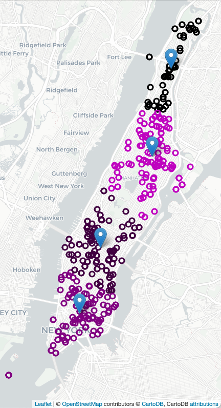
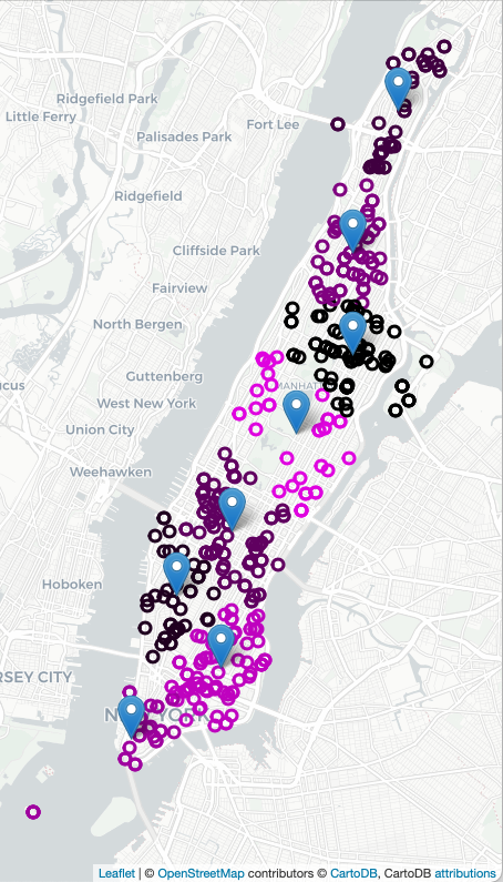
To decide on where to "pre-place" ambulances, we will start with K-means clustering, where "K" is the number of ambulances available for that shift. For example, if there 2 ambulances available to be placed in Manhattan, we will look at previous ambulance calls for that shift and form 2 clusters and station each ambulance at the mean of the cluster. If two more ambulances become available, we can recompute the K-means algorithm for K=4, and place those 4 ambulances, each at the mean of the cluster found, and similarly for K=8:

In addition to K-means analysis, we will also compare to other clustering techniques and use standard approaches from sklearn as well as filter data by time and day.

The program follows standard strategy for data cleaning and model building:

Read in datasets, merging and cleaning as needed.
Split our dataset into training and testing sets.
Fit a model, or multiple models, to the training dataset.
Validate the models using the testing dataset.
Develop test suites, using pytest, to ensure that correctness of the code written.

To download test datasets, see Program 2 for directions on accessing datasets at NYC Open Data.

Preparing Data

Once you have downloaded some test data sets to your device, the next thing to do is format the data to be usable for analysis. We will need to do some cleaning, and also filter by day of week and time. Once we have the cleaned the data, we can split it into training and testing data sets. Add the following functions to your Python program:

make_df(file_name): This function takes one input:
- file_name: the name of a CSV file containing 911 System Calls from OpenData NYC.
The data is read into a DataFrame. Rows that are have null values for the type description, incident date, incident time, latitute and longitude are dropped. Only rows that contain AMBULANCE as part of the TYP_DESC are kept. The resulting DataFrame is returned.
Hint: see DS 100: Chapter 13 for using string methods within pandas.
See Classwork 9.
add_date_time_features(df): This function takes one input:
- df: a DataFrame containing 911 System Calls from OpenData NYC created by make_df.
An additional column WEEK_DAY is added with the day of the week (0 for Monday, 1 for Tuesday, ..., 6 for Sunday) of the date in INCIDENT_DATE is added. Another column, INCIDENT_MIN, that takes the time from INCIDENT_TIME and stores it as the number of minutes since midnight. The resulting DataFrame is returned.
Hint: see Lecture 3 for using datetime methods with pandas, including computing the day of the week (of datetime objects) and the total seconds (of timedelta objects).
filter_by_time(df, days=None, start_min=0, end_min=1439): This function takes four inputs:
- df: a DataFrame containing 911 System Calls from OpenData NYC.
- days: a list of integers ranging from 0 to 6, representing the days of the week. The default value is None and is equivalent to the list containing all days: [0,1,2,3,4,5,6].
- start_min: a non-negative integer value representing the starting time. With end_min, it representing the range, inclusive, for the time, in minutes, that should be selected. The default value give the range of [0,1439] which ranges from midnight (0 minutes) to (1439 representing 23:59 since 23 hours + 59 minutes = 23*60+59 minutes = 1439 minutes).
- end_min: a non-negative integer value representing the ending time. With start_min, it representing the range, inclusive, for the time, in minutes, that should be selected. The default value give the range of [0,1439] which ranges from midnight (0 minutes) to (1439 representing 23:59 since 23 hours + 59 minutes = 23*60+59 minutes = 1439 minutes).
Returns a DataFrame with entries restricted to weekdays in days (or all weekdays if None is given) and incident times in [start_min, end_min] inclusive (e.g. contains the endpoints).

For example, if we use the small dataset from 4 July 2021:

df = make_df('NYPD_Calls_Manhattan_4Jul2021.csv')
print(df[['INCIDENT_TIME','TYP_DESC','Latitude','Longitude']])

would print:

     INCIDENT_TIME                             TYP_DESC   Latitude  Longitude
7         00:01:51      AMBULANCE CASE: CARDIAC/OUTSIDE  40.724578 -73.992519
27        00:06:12       AMBULANCE CASE: CARDIAC/INSIDE  40.807719 -73.964240
51        00:12:12      AMBULANCE CASE: SERIOUS/TRANSIT  40.732019 -74.000734
53        00:12:38           AMBULANCE CASE: EDP/INSIDE  40.789348 -73.947352
54        00:12:38           AMBULANCE CASE: EDP/INSIDE  40.789348 -73.947352
...            ...                                  ...        ...        ...
5175      23:50:02         AMBULANCE CASE: WATER RESCUE  40.711839 -74.011234
5176      23:50:02         AMBULANCE CASE: WATER RESCUE  40.711839 -74.011234
5205      23:57:11  AMBULANCE CASE: UNCONSCIOUS/TRANSIT  40.732019 -74.000734
5211      23:57:59           AMBULANCE CASE: EDP/INSIDE  40.827547 -73.937461
5212      23:57:59           AMBULANCE CASE: EDP/INSIDE  40.827547 -73.937461

[459 rows x 4 columns]

Note that the original CSV file had over 5000 lines, only 459 of those were for ambulances calls. The indices were not reset and refer to the line numbers of the original file.

Let's add in the date and time features:

df = add_date_time_features(df)
print(df[['INCIDENT_DATE','WEEK_DAY','INCIDENT_TIME','INCIDENT_MIN']])

would print:

     INCIDENT_DATE  WEEK_DAY INCIDENT_TIME  INCIDENT_MIN
7       07/04/2021         6      00:01:51      1.850000
27      07/04/2021         6      00:06:12      6.200000
51      07/04/2021         6      00:12:12     12.200000
53      07/04/2021         6      00:12:38     12.633333
54      07/04/2021         6      00:12:38     12.633333
...            ...       ...           ...           ...
5175    07/04/2021         6      23:50:02   1430.033333
5176    07/04/2021         6      23:50:02   1430.033333
5205    07/04/2021         6      23:57:11   1437.183333
5211    07/04/2021         6      23:57:59   1437.983333
5212    07/04/2021         6      23:57:59   1437.983333

[459 rows x 4 columns]
[Finished in 2.294s]

Since all the incidents are from a single day (i.e. 4 July 2021) the WEEK_DAY column has the same value (i.e. 6) for every row.

Let's add in the date and time features:

df_early_am = filter_by_time(df,times=[0,360])
print(df_early_am[['INCIDENT_DATE','WEEK_DAY','INCIDENT_TIME','INCIDENT_MIN']])

would print:

     INCIDENT_DATE  WEEK_DAY INCIDENT_TIME  INCIDENT_MIN
7       07/04/2021         6      00:01:51      1.850000
27      07/04/2021         6      00:06:12      6.200000
51      07/04/2021         6      00:12:12     12.200000
53      07/04/2021         6      00:12:38     12.633333
54      07/04/2021         6      00:12:38     12.633333
...            ...       ...           ...           ...
1041    07/04/2021         6      05:08:49    308.816667
1068    07/04/2021         6      05:21:49    321.816667
1075    07/04/2021         6      05:24:21    324.350000
1079    07/04/2021         6      05:28:13    328.216667
1111    07/04/2021         6      05:41:34    341.566667

[76 rows x 4 columns]

We can build a map with the calls for ambulances shaded by the time of the call:

import folium
import matplotlib.colors
def cc(minute,scale):
    return(matplotlib.colors.to_hex( (minute/scale,0,minute/scale) ))

m = folium.Map(location=[40.7678,-73.9645],zoom_start=13,tiles="cartodbpositron")
df.apply( lambda row: folium.CircleMarker(location=[row["Latitude"], row["Longitude"]],
                                        radius=5, popup=(row['INCIDENT_TIME']+": "+row['TYP_DESC']),
                                        color=cc(row['INCIDENT_MIN'],2000))
                                        .add_to(m) ,
        axis=1)
m.save('4_July_map.html')

displayed above. Note that we used the time to shade the incidents. The popups provide the exact time as well as the description.

Building Models

Next, let's build some models, using the clustering techniques from Lecture 11. Write the following functions:

compute_kmeans(df, num_clusters = 8, n_init = 'auto', random_state = 1870): This function takes four inputs:
- df: a DataFrame containing 911 System Calls from OpenData NYC.
- n_init: Number of times the k-means algorithm is run with different centroid seeds. The final results is the best output of n_init consecutive runs in terms of inertia. The default value is auto.
- num_clusters: an integer representing the number of clusters. The default value is 8.
- random_state: the random seed used for KMeans. The default value is 1870.
Runs the KMeans model with num_clusters on the latitude and longitude data of the provided DataFrame. Returns the cluster centers and predicted labels computed via the model.
A similar, but not identical function was part of Classwork 9.
compute_gmm(df, num_clusters = 8, random_state = 1870): This function takes three input:
- df: a DataFrame containing 911 System Calls from OpenData NYC.
- num_clusters: an integer representing the number of clusters. The default value is 8.
- random_state: the random seed used for GaussianMixture. The default value is 1870.
Runs the GaussianMixture model with num_clusters on the latitude and longitude data of the provided DataFrame. Returns the array of the predicted labels computed via the model.
compute_agglom(df, num_clusters = 8, linkage='ward'): This function takes three inputs:
- df: a DataFrame containing 911 System Calls from OpenData NYC.
- num_clusters: an integer representing the number of clusters. The default value is 8.
- linkage: the linkage criterion used determining distances between sets for AgglomerativeClustering. The default value is 'ward'.
Runs the Agglomerative model with num_clusters on the latitude and longitude data of the provided DataFrame and default linkage (i.e. ward). Returns the array of the predicted labels computed via the model.
compute_spectral(df, num_clusters = 8, affinity='rbf',random_state=1870): This function takes four inputs:
- df: a DataFrame containing 911 System Calls from OpenData NYC.
- num_clusters: an integer representing the number of clusters. The default value is 8.
- affinity: method used for computing the affinity matrix by SpectralClustering. The default value is 'rbf'.
- random_state: the random seed used for SpectralClustering. The default value is 1870.
Runs the Spectral Clustering model with num_clusters on the latitude and longitude data of the provided DataFrame and affinity matrix (i.e. affinity). Returns the array of the predicted labels computed via the model.

We can also make maps with the computed clusters. We use the compute_locations function with different values of num_clusters. Since we are repeating the same actions for K = 2, 4, 6, we wrote a helper function to create the HTML maps:

def make_map(df, num_clusters, out_file):
            centers,labels = compute_kmeans(df,num_clusters = num_clusters)
            df_map = df[ ['Latitude','Longitude','INCIDENT_TIME','INCIDENT_MIN','TYP_DESC'] ]
            df_map = df_map.assign(Labels = labels)
            m = folium.Map(location=[40.7678,-73.9645],zoom_start=13,tiles="cartodbpositron")
            df_map.apply( lambda row: folium.CircleMarker(location=[row["Latitude"], row["Longitude"]],
                                                radius=5, popup=(row['INCIDENT_TIME']+": "+row['TYP_DESC']),
                                                color=cc(row['Labels'],num_clusters))
                                                .add_to(m), axis=1)
            for i in range(num_clusters):
                x,y = centers[i]
                folium.Marker(location=[x,y],popup = "Cluster "+str(i)).add_to(m)
            m.save(out_file)
        
        make_map(df,2,'map_4_July_2clusters.html')
        make_map(df,4,'map_4_July_4clusters.html')
        make_map(df,8,'map_4_July_8clusters.html')

Screenshots of the maps are displayed above.

Another function can be used to filter the dataset by day of the week and time of day. For example, still working with the 4 July data set:

df_mondays = filter_by_time(df, days = [0])
        print(df_mondays)

This will return an empty DataFrame since only 4 of July in this data set (which was a Sunday and we filtered for 0 or Monday):

Empty DataFrame
        Columns: [CAD_EVNT_ID, CREATE_DATE, INCIDENT_DATE, INCIDENT_TIME, NYPD_PCT_CD, BORO_NM, PATRL_BORO_NM, GEO_CD_X, GEO_CD_Y, RADIO_CODE, TYP_DESC, CIP_JOBS, ADD_TS, DISP_TS, ARRIVD_TS, CLOSNG_TS, Latitude, Longitude, WEEK_DAY, INCIDENT_MIN]
        Index: []

Let's next filter for early morning times:

df_early_am = filter_by_time(df,times=[0,360])
        print(df_early_am[['INCIDENT_DATE','WEEK_DAY','INCIDENT_TIME','INCIDENT_MIN']])

would print:

     INCIDENT_DATE  WEEK_DAY INCIDENT_TIME  INCIDENT_MIN
        7       07/04/2021         6      00:01:51      1.850000
        27      07/04/2021         6      00:06:12      6.200000
        51      07/04/2021         6      00:12:12     12.200000
        53      07/04/2021         6      00:12:38     12.633333
        54      07/04/2021         6      00:12:38     12.633333
        ...            ...       ...           ...           ...
        1041    07/04/2021         6      05:08:49    308.816667
        1068    07/04/2021         6      05:21:49    321.816667
        1075    07/04/2021         6      05:24:21    324.350000
        1079    07/04/2021         6      05:28:13    328.216667
        1111    07/04/2021         6      05:41:34    341.566667
        
        [76 rows x 4 columns]

We can use other methods for clustering, printing out the labels for the uly 4 dataset:

print(compute_gmm(df))
        print(compute_agglom(df))

[1 7 1 0 0 1 1 0 0 4 0 2 1 5 5 2 2 1 1 4 4 4 4 5 1 6 3 5 3 3 7 0 7 1 3 3 3
        3 1 2 2 7 6 1 1 1 2 0 0 4 5 3 4 6 6 3 1 3 3 1 6 4 6 0 6 6 3 2 6 3 1 1 1 1
        4 4 5 2 1 2 2 7 7 1 1 5 3 1 0 5 5 4 4 2 0 0 0 0 2 2 4 4 3 1 1 7 4 3 3 6 6
        2 1 0 3 3 1 5 5 2 3 3 1 1 5 5 2 2 0 2 2 3 2 2 1 5 5 1 5 0 0 0 2 2 1 1 5 2
        1 3 0 5 5 5 1 1 2 0 0 7 7 7 6 6 3 3 4 4 1 1 1 1 1 3 1 7 4 4 0 1 5 1 3 7 0
        4 4 3 1 3 3 0 0 0 0 1 1 1 6 6 0 0 0 0 5 2 2 5 5 3 4 4 1 4 2 0 2 0 2 2 1 1
        1 3 3 1 3 3 1 0 0 5 5 1 5 5 1 7 5 2 1 0 0 0 1 5 2 0 2 1 4 4 1 1 4 7 7 3 3
        4 1 1 7 7 5 5 0 1 5 1 1 0 7 0 0 2 0 7 7 5 1 2 3 1 1 1 1 3 6 6 4 5 5 2 2 0
        3 0 0 2 5 5 0 1 3 7 7 5 5 3 0 6 0 0 1 2 4 5 2 1 3 3 1 1 2 0 1 2 2 2 3 3 4
        4 5 5 1 2 0 3 4 3 3 0 1 6 1 1 4 1 4 4 3 6 6 6 2 2 2 3 6 3 3 1 0 5 3 5 2 2
        3 3 6 6 2 2 3 6 6 2 0 0 3 3 2 0 3 2 2 3 3 4 4 6 6 1 6 4 5 5 5 4 6 1 1 1 4
        2 0 3 5 2 1 3 1 4 3 1 0 3 5 5 5 3 3 7 3 1 2 2 2 4 4 2 2 2 1 1 3 3 2 3 5 1
        1 1 0 0 0 0 4 4 5 6 6 6 1 2 2]
        [0 6 0 3 3 0 0 3 3 2 3 4 0 7 7 4 4 0 0 2 2 2 2 7 0 0 1 0 1 1 6 3 1 0 1 1 1
        1 0 4 4 4 5 0 0 0 4 3 3 2 3 1 2 0 0 1 0 1 1 0 0 2 0 3 0 0 1 4 0 1 0 0 0 0
        2 2 3 4 0 4 4 1 1 1 0 3 1 0 3 7 7 2 2 4 3 3 3 3 4 4 2 2 1 0 0 6 2 1 1 0 0
        4 0 4 1 1 0 0 0 4 1 1 0 0 7 7 4 4 3 4 4 1 4 4 0 7 7 0 7 3 3 3 4 4 0 0 7 4
        0 1 3 7 0 0 0 0 4 3 3 6 6 4 5 5 1 1 2 2 0 0 0 0 0 1 0 6 2 2 3 0 7 0 1 6 3
        2 2 1 0 0 0 3 3 3 3 0 0 0 0 5 3 3 3 3 7 4 4 7 7 1 2 2 0 4 4 3 4 6 4 4 0 0
        0 1 1 0 1 1 0 3 3 7 7 0 3 3 0 6 3 4 0 3 3 3 0 7 4 3 4 0 2 4 0 0 2 6 6 1 1
        2 0 0 6 6 3 3 3 0 7 5 5 3 6 3 3 4 3 6 6 0 0 4 1 0 0 0 0 1 5 5 2 7 7 4 4 3
        1 3 3 4 7 7 3 0 1 6 6 7 7 7 3 0 3 3 0 4 2 7 4 0 1 1 1 1 4 3 0 4 4 4 1 1 2
        2 0 0 0 4 3 1 2 1 1 3 0 5 0 0 2 0 2 2 1 5 5 5 4 4 4 1 5 1 1 0 3 7 1 3 4 4
        1 1 5 5 4 4 1 0 0 4 3 3 1 1 4 3 1 4 4 1 1 2 2 5 5 0 5 2 7 3 3 2 5 0 0 0 2
        4 4 1 7 4 0 1 0 2 1 0 3 1 7 3 3 1 1 6 1 0 4 4 4 2 2 4 4 4 0 0 1 1 4 1 3 0
        0 0 3 3 3 3 2 2 3 5 5 5 0 4 4]

Evaluating Models

compute_explained_variance(df, k_vals = None, random_state = 1870): This function takes three inputs:
- df: a DataFrame containing 911 System Calls from OpenData NYC.
- k_vals: a list of integers representing values for the number of clusters. The no value is provided, the function uses k_vals = [1,2,3,4,5].
- random_state: the random seed used for KMeans. The default value is 55.
Returns a list of the sum of squared distances of samples to their closest cluster center for each value of K. This can be computed manually or via the inertia_ attribute of the KMeans model.

We can use the function compute_explained_variance to assess the best number of clusters:

k_vals = list(range(1,20))
ev = compute_explained_variance(df,K=k_vals)
sns.lineplot(k_vals,ev)
plt.title('Explained Variance for KMeans for Manhattan, 4 July 2021')
plt.show()

will display:

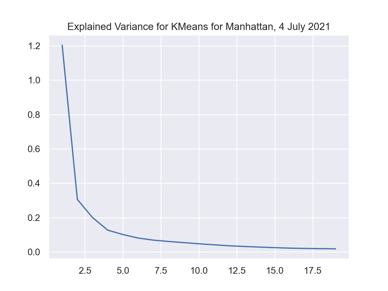
showing a sharp drop-off to K=5 that quickly flattens, showing that additional clusters, beyond 10, do not significantly improve the average distance to the assigned means. This suggests that a reasonable number of clusters is around 8.

Test Suites

Each programming assignment includes functions that test that your code works (a "test suite"). In Programs 1 & 2, we wrote the test functions by hand. For Programs 3-6, we will also use pytest, a standard Python testing framework. Before you start, make sure that your IDE has pytest installed:

pip install -U pytest

Pytest is one of the most popular testing frameworks for Python. For this program, we will introduce the core testing features (and will introduce more features, such as parametrizing, in future programs). For more details, see Lecture 5, pytest docs and Think CS: Chapter 20.

test_add_date_time_features(): This function takes no inputs. Returns True if the function add_date_time_features performs correctly and False otherwise.

test_filter_by_time(): This function takes no inputs. Returns True if the function filter_by_time performs correctly and False otherwise.

Trying first on the correct function, assuming that your program is called p5.py, we can invoke pytest from the command-line:

pytest p5.py::test_add_date_time_features

gives the output:

======================================= test session starts ========================================
  platform darwin -- Python 3.11.5, pytest-7.4.2, pluggy-1.3.0
  rootdir: /Users/stjohn/gitHub/dataScience/programs/fall23/program05
  collected 1 item                                                                                   
  
  p5.py .                                                                                      [100%]
  
  ======================================== 1 passed in 1.63s =========================================

pytest looks for a function called: test_add_date_time_features() in the file p3.py. It then runs test_add_date_time_features, which tests the correctness of the function add_date_time_features and reports back the results.

Program 5: EMS Clusters CSci 39542: Introduction to Data Science Department of Computer Science Hunter College, City University of New York Fall 2023

Program Description

Preparing Data

Building Models

Evaluating Models

Test Suites

Program 5: EMS Clusters
CSci 39542: Introduction to Data Science
Department of Computer Science
Hunter College, City University of New York
Fall 2023