Program 6: EMS Queries
CSci 39542: Introduction to Data Science
Department of Computer Science
Hunter College, City University of New York
Fall 2023
Classwork Quizzes Homework Project
Program Description
Program 6: EMS Queries. Due noon, Friday, 8 December.
This program continues the analysis of the emergency services calls that was introduced in Program 5. It follows standard strategy for data cleaning and model building, with the focus on using SQL for exploratory data analys.
To download test datasets, see Program 5. Once you have downloaded some test data sets to your device, the next thing to do is format the data to be usable for analysis. We will need to do some cleaning, and also filter by day of week and time. Once we have the cleaned the data, we can split it into training and testing data sets. Add the following functions to your Python program: For example, if we use the dataset of midnight calls from January 2021:
We can add a new column that has the time taken to dispatch services, by applying the
We will be using Structured Query Language (SQL) to subset and aggregate data (see Lectures 25 & 26 and DS 100: Chapter 7). For this program, we will use the pandasql that provides an easy way to query pandas DataFrames using SQL syntax. To use it, you may need to install it on your machine (e.g.
Once installed, you can run queries via the function Note that strings need to be surrounded by quotes in your query
(e.g. Note that The first function uses SQL to select the column containing the borough name:
The next function, takes the DataFrame and the name of a borough and uses SQL to select all rows with that borough name. For example, we can select We can use SQL to calculate how many incidents were called in on New Year's Day in Queens:
We can calculate summary counts for the DataFrame:
As well which are the 10 most common for Brooklyn and Staten Island:
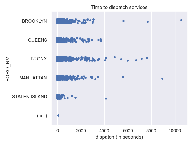
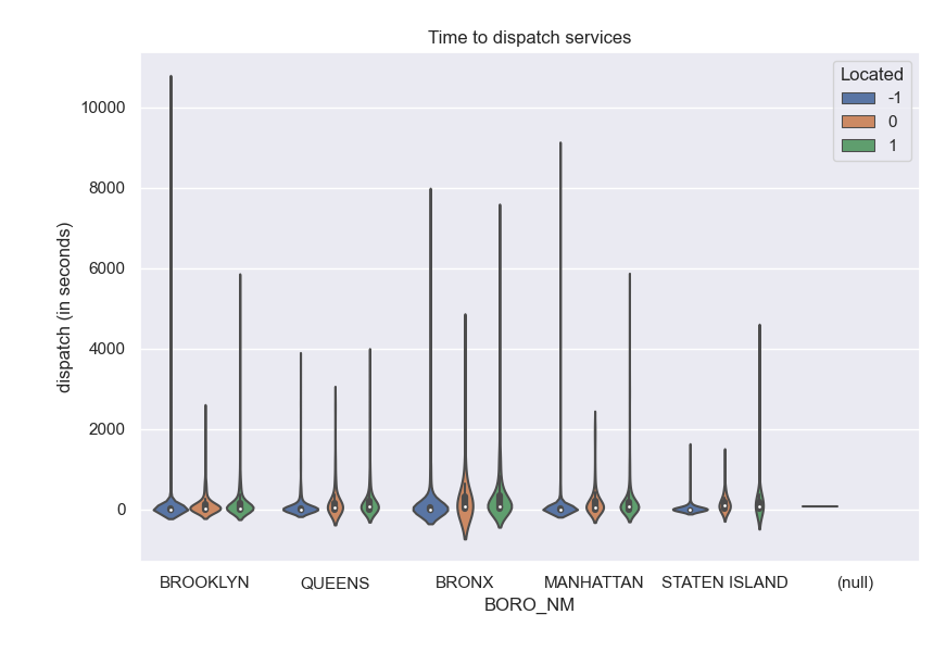
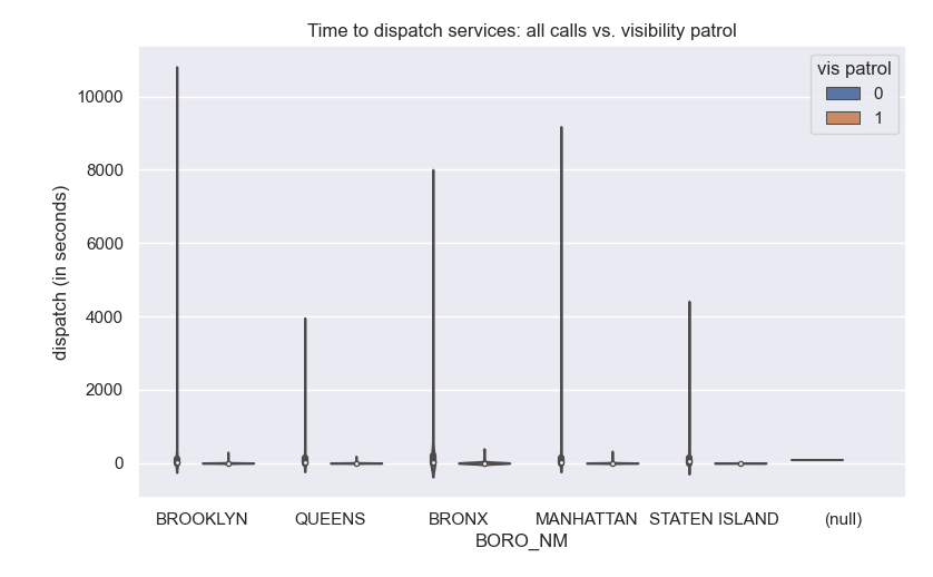
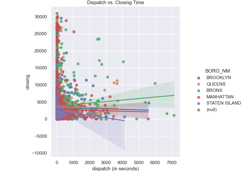
Let's use seaborn to visualize both the time taken to complete. Since we have many similar data points, we will use the Many of the descriptions include if there are inside or outside the address. Let's use seaborn's violin plot to see if the location makes a difference in how quickly emergency services are dispatched: The SQL queries highlighted the most common calls for emergency services is "visibility patrol". We can use seaborn's linear model visualization to show the differences in response time between boroughs:
Learning Objective: To reinforce new SQL skills to query and aggregate data.
Available Libraries: pandas, pandasql, and core Python 3.6+.
Data Sources: 911 System Calls (NYC OpenData)
Sample Datasets:
Preparing Data
make_df(file_name):
This function takes one input:
The data is read into a DataFrame. Rows that are have null values for the type description, incident date, incident time, borough name are dropped.
The resulting DataFrame is returned.
file_name: the name of a CSV file containing 911 System Calls from OpenData NYC.
Hint: this is slightly different than the function from Program 5 in that different rows are dropped and it does not restrict to only ambulance calls.
compute_time_delta(start, stop):
This function takes two inputs:
The function converts the input strings into start: a string containing a date/time in the format:
MM/DD/YYYY HH:MM:SS XM with month, day, year, hour, minutes, and seconds as digits and XM either AM or PM.
stop: a string containing a date/time in the format:
MM/DD/YYYY HH:MM:SS XM with month, day, year, hour, minutes, and seconds as digits and XM either AM or PM.
datetime objects and returns a whole number that is the difference in time in seconds.
Note: instead of taking a Series or DataFrame as an argument, this function is applied to a DataFrame. See the example below.
would print:
df = make_df('NYPD_Calls_midnight_Jan2021.csv')
print(df[['BORO_NM','RADIO_CODE','TYP_DESC']]) BORO_NM RADIO_CODE TYP_DESC
0 BROOKLYN 10S2 INVESTIGATE/POSSIBLE CRIME: SHOTS FIRED/OUTSIDE
1 QUEENS 68Q1 SEE COMPLAINANT: OTHER/INSIDE
2 BRONX 54E1 AMBULANCE CASE: EDP/INSIDE
3 BRONX 54E1 AMBULANCE CASE: EDP/INSIDE
4 BROOKLYN 24Q6 ASSAULT (PAST): OTHER/FAMILY
... ... ... ...
5582 MANHATTAN 54E1 AMBULANCE CASE: EDP/INSIDE
5583 MANHATTAN 54E1 AMBULANCE CASE: EDP/INSIDE
5584 MANHATTAN 75D VISIBILITY PATROL: DIRECTED
5585 BROOKLYN 75D VISIBILITY PATROL: DIRECTED
5586 QUEENS 75D VISIBILITY PATROL: DIRECTED
[5587 rows x 3 columns]compute_time_delta function to the DataFrame:
which yields:
df['dispatch (in seconds)'] = df.apply(lambda row: compute_time_delta(row['ADD_TS'],row['DISP_TS']),axis='columns')
print(df[['INCIDENT_DATE','BORO_NM','dispatch (in seconds)']]) INCIDENT_DATE BORO_NM dispatch (in seconds)
0 01/01/2021 BROOKLYN 31
1 01/01/2021 QUEENS 0
2 01/01/2021 BRONX 32
3 01/01/2021 BRONX 62
4 01/01/2021 BROOKLYN 644
... ... ... ...
5582 02/01/2021 MANHATTAN 13
5583 02/01/2021 MANHATTAN 10
5584 02/01/2021 MANHATTAN 0
5585 02/01/2021 BROOKLYN 0
5586 02/01/2021 QUEENS 1
[5587 rows x 3 columns]
Using SQL with Pandas
pip install pandasql or pip3q install pandasql). See pandasql for installation details.
sqldf(queryName). For example, you could filter for all the neighborhood tabulation areas in the Bronx in the NYC_population_by_NTA.csv on the waitlist by:
which prints:
import pandas as pd
import pandasql as psql
pop = pd.read_csv('NYC_population_by_NTA.csv')
q = 'SELECT * FROM pop WHERE Borough = "Bronx"'
bronx = psql.sqldf(q)
print(bronx.head()) Borough Year ... NTA Name Population
0 Bronx 2000 ... Claremont-Bathgate 28149
1 Bronx 2000 ... Eastchester-Edenwald-Baychester 35422
2 Bronx 2000 ... Bedford Park-Fordham North 55329
3 Bronx 2000 ... Belmont 25967
4 Bronx 2000 ... Bronxdale 34309
[5 rows x 6 columns]"Waitlist Student"). To set up your queries, you may find Formatted Literal Strings ("f-strings") useful (see the python tutorial or Lecture 2 for more details).pandasql uses the DataFrames that are given in the query, without the DataFrames being passed in as arguments. This causes issues with pylint since the DataFrame looks unused. There are several ways to tell pylint that a variable is necessary but not used explicitly. In the functions below, we use leading underscores for the DataFrame names (e.g. _df) to signal that it is a necessary variable but used internally.
select_boro_column(_df):
This function takes one input:
Selects, using SQL, the _df: a DataFrame containing 911 System Calls from OpenData NYC created by make_df.
BORO_NM column from _df.
Returns the resulting DataFrame from the SQL query.
select_by_boro(df, boro_name):
This function takes two inputs:
Selects, using SQL, all rows from the DataFrame, _df: a DataFrame containing 911 System Calls from OpenData NYC created by make_df.
boro_name: a string containing the name of a borough. Can be lower or upper case.
_df, where the borough is boro_name.
Returns the resulting DataFrame from the SQL query.
Hint: Since the boro_name can be upper or lower case, convert it to upper case to match the way the borough names are stored.
new_years_count(_df, boro_name):
This function takes two inputs:
Selects, using SQL, the number of incidents from _df: a DataFrame containing 911 System Calls from OpenData NYC created by make_df.
boro_name: a string containing the name of a borough. Can be lower or upper case.
_df, called in on New Year's Day (Jan 1, 2021) in the specified borough, boro_name.
Returns the resulting DataFrame from the SQL query.
Hint: Since the boro_name can be upper or lower case, convert it to upper case to match the way the borough names are stored.
incident_counts(_df):
This function takes one inputs:
Selects, using SQL, the incident counts per radio code (_df: a DataFrame containing 911 System Calls from OpenData NYC created by make_df.
TYP_DESC), sorted alphabetically by radio code (TYP_DESC). Returns the resulting DataFrame from the SQL query.
top_10(_df, boro_name):
This function takes two inputs:
Selects, using SQL, the top 10 most commonly occurring incidence by radio code, and the number of incident occurrences, in specified borough. Returns the resulting DataFrame from the SQL query.
_df: a DataFrame containing 911 System Calls from OpenData NYC created by make_df.
boro_name: a string containing the name of a borough. Can be lower or upper case.
Hint: Since the boro_name can be upper or lower case, convert it to upper case to match the way the borough names are stored.
would print:
boros = select_boro_column(df)
print(boros) BORO_NM
0 BROOKLYN
1 QUEENS
2 BRONX
3 BRONX
4 BROOKLYN
... ...
5582 MANHATTAN
5583 MANHATTAN
5584 MANHATTAN
5585 BROOKLYN
5586 QUEENS
[5587 rows x 1 columns]Bronx
would print:
df_bx = select_by_boro(df, "Bronx")
print(df_bx) CAD_EVNT_ID CREATE_DATE ... Latitude Longitude
0 73973992 01/01/2021 ... 40.830860 -73.902887
1 73973992 01/01/2021 ... 40.830860 -73.902887
2 73974010 01/01/2021 ... 40.840868 -73.925150
3 73974019 01/01/2021 ... 40.870439 -73.890847
4 73974033 01/01/2021 ... 40.856654 -73.843872
... ... ... ... ... ...
1007 74629410 02/01/2021 ... 40.859192 -73.900677
1008 74629421 02/01/2021 ... 40.834562 -73.915443
1009 74630917 02/01/2021 ... 40.825472 -73.892941
1010 74642928 02/01/2021 ... 40.859640 -73.863235
1011 74643746 02/01/2021 ... 40.870371 -73.851975
[1012 rows x 18 columns]
would print:
df_nyd_q = new_years_count(df, "Queens")
print(df_nyd_q) COUNT(*)
0 40
would print:
df_inc = incident_counts(df)
print(df_inc) TYP_DESC COUNT(*)
0 ALARMS: AUDIBLE/INSIDE 1
1 ALARMS: AUDIBLE/OUTSIDE 6
2 ALARMS: AUDIBLE/TRANSIT 5
3 ALARMS: BANK/BURGLARY 3
4 ALARMS: COMMERCIAL/BURGLARY 146
.. ... ...
181 VISIBILITY PATROL: DIRECTED 1334
182 VISIBILITY PATROL: FAMILY/HOME VISIT 44
183 VISIBILITY PATROL: INTERIOR 61
184 VISIBILITY PATROL:PUBLIC/PRIVATE EDUCATIONAL F... 4
185 YOUTH HOME VISIT 5
[186 rows x 2 columns]
would print:
df_si = top_10(df, "Staten Island")
print('Top 10 for Staten Island:')
print(df_si)
df_bk = top_10(df, "Brooklyn")
print('\nTop 10 for Brooklyn:')
print(df_bk)Top 10 for Staten Island:
TYP_DESC COUNT(*)
0 VISIBILITY PATROL: DIRECTED 97
1 COMMUNITY TIME 19
2 SEE COMPLAINANT: OTHER/INSIDE 18
3 AMBULANCE CASE: EDP/INSIDE 10
4 INVESTIGATE/POSSIBLE CRIME: SERIOUS/OTHER 8
5 DISPUTE: INSIDE 8
6 BUS INVESTIGATION 7
7 AMBULANCE CASE: SERIOUS/INSIDE 7
8 DISPUTE: FAMILY 5
9 DISORDERLY: GROUP/OUTSIDE 5
Top 10 for Brooklyn:
TYP_DESC COUNT(*)
0 VISIBILITY PATROL: DIRECTED 503
1 STATION INSPECTION BY TRANSIT BUREAU PERSONNEL 189
2 SEE COMPLAINANT: OTHER/INSIDE 189
3 TRAIN RUN/MOBILE ORDER MAINTENANCE SWEEP 72
4 AMBULANCE CASE: EDP/INSIDE 60
5 INVESTIGATE/POSSIBLE CRIME: SUSP VEHICLE/OUTSIDE 52
6 INVESTIGATE/POSSIBLE CRIME: CALLS FOR HELP/INSIDE 48
7 ALARMS: COMMERCIAL/BURGLARY 44
8 VISIBILITY PATROL: INTERIOR 39
9 INVESTIGATE/POSSIBLE CRIME: SERIOUS/OTHER 36
Building Models
sns.stripplot which "jitters" the points to highlight the density:
which gives the plot:
sns.stripplot(data=df,x="dispatch (in seconds)",y="BORO_NM")
plt.title('Time to dispatch services')
plt.tight_layout()  #for nicer margins
plt.show()
which gives the plot:
def locate_fnc(desc):
  if "INSIDE" in desc:
      return 1
  if "OUTSIDE" in desc:
      return 0
  return -1
df["Located"] = df["TYP_DESC"]apply(locate_fnc)
sns.violinplot(data=df, x="BORO_NM", y="dispatch (in seconds)",hue="Located")
plt.title('Time to dispatch services')
plt.tight_layout()  #for nicer margins
plt.show()
which gives the plots:
sns.violinplot(data=df, x="BORO_NM", y="dispatch (in seconds)",hue="vis patrol")
plt.title('Time to dispatch services: all calls vs. visibility patrol')
plt.tight_layout()  #for nicer margins
plt.show()

df['closing'] = df.apply(lambda row: compute_time_delta(row['DISP_TS'],row['CLOSNG_TS']),axis='columns')
ax=sns.lmplot(data=df[(df['dispatch (in seconds)'] <= 60*60*2) & (df['closing'] <= 60*60*12)], \
  x="dispatch (in seconds)",y="closing",hue="BORO_NM")
plt.title('Dispatch vs. Closing Time')
plt.show() 
