Coursework
CSci 39542: Introduction to Data Science
Department of Computer Science
Hunter College, City University of New York
Spring 2022
Classwork Quizzes Homework Project
Classwork
Unless otherwise noted, classwork is submitted via Gradescope. Access information is given during the corresponding lecture.
Due to the internet issues in the lecture hall, for Classwork 2 onward, the classwork will be available until midnight. If you attended class that day, there is an option to earn 0.5 points for attendance and space to include the row and seat number. If you were not able to attend a given lecture, you can still work through the classwork at home and we will replace the fractional point for that classwork with the grade you earned on the final exam. Do not say you were in the room if you did not attend.
- First, the attendance is used in case of contact tracing for covid. The college and health officials need an accurate information for isolation and quarantine planning. You will have to explain your misrepresenting your class presense to the department chair, the dean, and the administrators responsible for student affairs and health, as well as possible isolation for you and your close contacts.
- Second, lying about attendance obtains an unfair advantage and will be submitted to the Office of Student Conduct. It is not worth 0.5 points (that would have been replaced anyway by your final exam score) for a record of academic dishonesty that is kept by both the department and college. The suggested sanction for lying is a 0 on this classwork and the loss of the replacement policy for missed lecture grades. Note: while we suggest a sanction, the final decision about the severity of the sanction is by the Office of Student Conduct.
Classwork 0: Due midnight, Monday, 31 January.
Available on Gradescope, this classwork focuses on the course
syllabus.
If you do have access to the course on Gradescope, write to datasci@hunter.cuny.edu. Include in your email that you not receive a Gradescope invitation, your preferred email, and we will manually generate an invitation.
Classwork 1: Due 4pm, Monday, 31 January.
Available during Lecture 1 on Gradescope (paper version also available for those without a phone or laptop at lecture), this classwork complements the exploratory data analysis of names and foreshadows the sampling of data in Lecture 2.
Classwork 2: Due midnight, Thursday, 3 February.
Available during Lecture 2 on Gradescope, this classwork introduces the autograder that is used for the programming assignments. The structure of the sample program mirrors the structure and content of the upcoming Program 1. To get the most out of this exercise, bring a laptop with you to lecture with a development environment (IDE) that has Python 3+ to work through in lecture. Write a function that takes the name of a file and makes a dictionary of the lines of the file.
For example, assuming these functions are in a file, Another example with nick_names.txt:
If you attended lecture, include the last three lines to the the introductory comment:
Classwork 3: Due midnight, Monday, 7 February.
Available during Lecture 3 on Gradescope, this classwork asks that you write a program using Pandas and its file I/O. To get the most out of this exercise, bring a laptop with you to lecture with a development environment (IDE) that has Python 3+ to work through in lecture.
Write a program that asks the user for the name of an input CSV file and the name of an output CSV file. The program should open the file name provided by the user.
Next, the program should select rows where the field
Then a sample run of the program:
Hints:
Classwork 4: Due midnight, Thursday, 10 February.
Available during Lecture 4 on HackerRank, this classwork introduces the timed coding environment used for quizzes. This classwork mirrors the structure and content of the upcoming Quiz 1.
To get the most out of this exercise, bring an electronic device on which you can easily type into a web-based IDE (possible on a phone, but much easier with the bigger screen and keyboards on some tablets and most laptops.
Classwork 5: Due midnight, Monday, 14 February.
Available during Lecture 5 on Gradescope, this classwork focuses on the structure and topics for the optional project, based on the project overview in lecture.
Classwork 6: Due midnight, Thursday, 17 February.
Available during Lecture 6 on Gradescope, this on-line assignment reviews the different ways to merge DataFrames in Pandas.
Classwork 7: Due midnight, Thursday, 24 February.
Available during Lecture 7 on Gradescope, this classwork introduces regular expressions for data cleaning. To get the most out of this exercise, bring a laptop with you to lecture with a development environment (IDE) that has Python 3+ to work through in lecture.
Write a program that asks the user for the name of an input HTML file and the name of an output CSV file. Your program should use regular expressions (see Chapter 12.4 for using the For example, if the input file is:
Classwork 8: Due midnight, Monday, 28 February.
Available during Lecture 6 on Gradescope, this classwork introduces the Use the date time functionality of Pandas to write the following functions:
For example, using the Seaborn's Green Taxi Data Set and assuming your functions are in the Using the function our second function:
Note: you should submit a file with only the standard comments at the top, this function, and any helper functions you have written. The grading scripts will then import the file for testing. Classwork 9: Due midnight, Thursday, 3 March.
Available during Lecture 9 on Gradescope, this classwork focuses on the GeoJSON format, including hands-on activity with GeoJSON visual editor. To get the most out of this exercise, bring a laptop with you to lecture with a development environment (IDE) that has Python 3+ to work through in lecture.
Quiz 1: Core Python Due 4pm, Friday, 11 February.
Link to access HackerRank available at the end of Lecture 4 (and posted on Blackboard).
Quiz 2: Pandas Basics Due 4pm, Friday, 11 February.
Link to access HackerRank available at the end of Lecture 4 (and posted on Blackboard).
Note: Hunter College is committed to all students having the technology needed for their courses. If you are in need of technology, see
Student Life's Support & Resources Page.
make_dict(file_name, sep=': '): Takes a name of a file, file_name and a delimiter sep. The default value is ': '. If a line of the file does not include sep, the line should be ignored. Otherwise, for each line, the string preceding the delimiter sep is the key, and the string after sep is the value. Your function returns the dictionary.
cw2.py and run on a file containing names that start with 'A', contacts.txt:
will print:
contacts = cw2.make_dict('contacts.txt')
who = 'CS Department'
print(f'Contact info for {who} is {contacts[who]}.')Contact info for CS Department is 10th Floor HN, x5213.
will print:
nick_names = cw2.make_dict('nick_names.txt', sep = ' ')
names = ['Beth','Lisa','Meg','Greta','Amy','Mia']
for n in names:
print(f'Full name for {n} is {nick_names[n]}.')Full name for Beth is Elizabeth.
Full name for Lisa is Elizabeth.
Full name for Meg is Margaret.
Full name for Greta is Margaret.
Full name for Amy is Amelia.
Full name for Mia is Amelia.
If you did not attend lecture, do not include the above lines.
"""
Name:  YOUR_NAME
Email: YOUR_EMAIL
Resources:  RESOURCES USED
I attended lecture today.
Row:  YOUR_ROW
Seat:  YOUR_SEAT
"""
Grade is equal to 3 and the Year is equal to 2019 and write all rows that match that criteria to a new CSV file.
where the file Enter input file name: school-ela-results-2013-2019.csv
Enter output file name: ela2013.csvschool-ela-results-2013-2019.csv is extracted from NYC Schools Test Results (and truncated version of roughly the first 1000 lines for testing). The first lines of the output file would be:
School,Name,Grade,Year,Category,Number Tested,Mean Scale Score,# Level 1,% Level 1,# Level 2,% Level 2,# Level 3,% Level 3,# Level 4,% Level 4,# Level 3+4,% Level 3+4
01M015,P.S. 015 ROBERTO CLEMENTE,3,2019,All Students,27,606,1,3.7,7,25.9,18,66.7,1,3.7,19,70.4
01M019, P.S. 019 ASHER LEVY,3,2019,All Students,24,606,0,0.0,8,33.3,15,62.5,1,4.2,16,66.7
01M020,P.S. 020 ANNA SILVER,3,2019,All Students,57,593,13,22.8,24,42.1,18,31.6,2,3.5,20,35.1
Grade column contains a mixtures of numbers (e.g. 3) and strings ("All Grades"), the column is stored as strings.
Note: Hunter College is committed to all students having the technology needed for their courses. If you are in need of technology, see
Student Life's Support & Resources Page.
re package in Python) to find all links in the input file and store the link text and URL as columns: Title and URL in the CSV file specified by the user. For the URL, strip off the leading https:// or http:// and any trailing slashes (/):
Then a sample run of the program:
<html>
<head><title>Simple HTML File</title></head>

<body>
  <p> Here's a link for <a href="http://www.hunter.cuny.edu/csci">Hunter CS Department</a>
  and for <a href="https://stjohn.github.io/teaching/data/fall21/index.html">CSci 39542</a>.  </p>

  <p> And for <a href="https://www.google.com/">google</a>
</body>
</html>
And the Enter input file name: simple.html
Enter output file name: links.csvlinks.csv would be:
Title,URL
Hunter CS Department,www.hunter.cuny.edu/csci
CSci 39542,stjohn.github.io/teaching/data/fall21/index.html
google,www.google.comdatetime package. To get the most out of this exercise, bring a laptop with you to lecture with a development environment (IDE) that has Python 3+ to work through in lecture.
tripTime(start,end): This function takes two variables of type datetime and returns the difference between them.
weekdays(df,col): This function takes a DataFrame, df, containing the column name, col, and returns a DataFrame containing only times that fall on a weekday (i.e. Monday through Friday).
cw6.py:
Would give output:
import seaborn as sns
taxi = sns.load_dataset('taxis')
print(taxi.iloc[0:10])
taxi['tripTime'] = taxi.apply(lambda x: cw6.tripTime(x['pickup'], x['dropoff']), axis=1)
print(taxi.iloc[0:10])
                pickup              dropoff  ...  pickup_borough  dropoff_borough
0  2019-03-23 20:21:09  2019-03-23 20:27:24  ...       Manhattan        Manhattan
1  2019-03-04 16:11:55  2019-03-04 16:19:00  ...       Manhattan        Manhattan
2  2019-03-27 17:53:01  2019-03-27 18:00:25  ...       Manhattan        Manhattan
3  2019-03-10 01:23:59  2019-03-10 01:49:51  ...       Manhattan        Manhattan
4  2019-03-30 13:27:42  2019-03-30 13:37:14  ...       Manhattan        Manhattan
5  2019-03-11 10:37:23  2019-03-11 10:47:31  ...       Manhattan        Manhattan
6  2019-03-26 21:07:31  2019-03-26 21:17:29  ...       Manhattan        Manhattan
7  2019-03-22 12:47:13  2019-03-22 12:58:17  ...       Manhattan        Manhattan
8  2019-03-23 11:48:50  2019-03-23 12:06:14  ...       Manhattan        Manhattan
9  2019-03-08 16:18:37  2019-03-08 16:26:57  ...       Manhattan        Manhattan

[10 rows x 14 columns]
                pickup              dropoff  ...  dropoff_borough        tripTime
0  2019-03-23 20:21:09  2019-03-23 20:27:24  ...        Manhattan 0 days 00:06:15
1  2019-03-04 16:11:55  2019-03-04 16:19:00  ...        Manhattan 0 days 00:07:05
2  2019-03-27 17:53:01  2019-03-27 18:00:25  ...        Manhattan 0 days 00:07:24
3  2019-03-10 01:23:59  2019-03-10 01:49:51  ...        Manhattan 0 days 00:25:52
4  2019-03-30 13:27:42  2019-03-30 13:37:14  ...        Manhattan 0 days 00:09:32
5  2019-03-11 10:37:23  2019-03-11 10:47:31  ...        Manhattan 0 days 00:10:08
6  2019-03-26 21:07:31  2019-03-26 21:17:29  ...        Manhattan 0 days 00:09:58
7  2019-03-22 12:47:13  2019-03-22 12:58:17  ...        Manhattan 0 days 00:11:04
8  2019-03-23 11:48:50  2019-03-23 12:06:14  ...        Manhattan 0 days 00:17:24
9  2019-03-08 16:18:37  2019-03-08 16:26:57  ...        Manhattan 0 days 00:08:20

[10 rows x 15 columns]
will give output:
taxi = sns.load_dataset('taxis')
weekdays = cw6.weekdays(taxi,'pickup')
print(weekdays.iloc[0:10])
note that rows 0,4,8, and 10 have been dropped from the original DataFrame since those corresponded to weekend days.
  pickup              dropoff  ...  pickup_borough  dropoff_borough
1   2019-03-04 16:11:55  2019-03-04 16:19:00  ...       Manhattan        Manhattan
2   2019-03-27 17:53:01  2019-03-27 18:00:25  ...       Manhattan        Manhattan
5   2019-03-11 10:37:23  2019-03-11 10:47:31  ...       Manhattan        Manhattan
6   2019-03-26 21:07:31  2019-03-26 21:17:29  ...       Manhattan        Manhattan
7   2019-03-22 12:47:13  2019-03-22 12:58:17  ...       Manhattan        Manhattan
9   2019-03-08 16:18:37  2019-03-08 16:26:57  ...       Manhattan        Manhattan
11  2019-03-20 19:39:42  2019-03-20 19:45:36  ...       Manhattan        Manhattan
12  2019-03-18 21:27:14  2019-03-18 21:34:16  ...       Manhattan        Manhattan
13  2019-03-19 07:55:25  2019-03-19 08:09:17  ...       Manhattan        Manhattan
14  2019-03-27 12:13:34  2019-03-27 12:25:48  ...       Manhattan        Manhattan

[10 rows x 14 columns]
datetime object (e.g. pd.to_datetime(start)) to use the functionality.
dt prefix, similar to .str similar to .str to use string methods and properties (e.g. dt.dayofweek).
See the Python Docs: date time functionality for more details.
Quizzes
Unless otherwise noted, quizzes focus on the corresponding programming assignment. The quizzes are 30 minutes long and cannot be repeated. They are available for the 24 hours after lecture and assess your programming skill using HackerRank. Access information for each quiz will be available under the Quizzes menu on Blackboard.
This first coding challenge focuses on reading and processing data from a file using core Python 3.6+ as in Program 1.
This is the first quiz using Pandas and focuses on manipulating and creating new columns in DataFrames as in Program 2.
Homework
Unless otherwise noted, programs are submitted on the course's Gradescope site and are written in Python. The autograders expect a .py file and do not accept iPython notebooks.
Also, to receive full credit, the code should be compatible with Python 3.6 (the default for the Gradescope autograders).
All students registered by Monday, 26 January are sent a registration invitation to the email on record on their Blackboard account. If you did not receive the email or would like to use a different account, write to datasci@hunter.cuny.edu. Include in your email that you not receive a Gradescope invitation, your preferred email, and we will manually generate an invitation. As a default, we use your name as it appears in Blackboard/CUNYFirst (to update CUNYFirst, see changing your personal information). If you prefer a different name for Gradescope, include it, and we will update the Gradescope registration.
To encourage starting early on programs, bonus points are given for early submission. A point a day, up to a total of 3 bonus points (10% of the program grade), are possible. The points are prorated by hour. For example, if you turn in the program 36 hours early, then the bonus poins are: (36 hours/3 days)*3 points = (36 hours/72 hours)*3 points = 1.5 points.
To get full credit for a program, the file must include in the opening comment:
- Your name, as it appears in your Gradescope registration.
- The email you are using for Gradescope.
- A list of any resources you used for the program. Include classmates and tutors that you worked with, along with any websites or tutorials that you used. If you used no resources (other than the class notes and textbooks), then you should include the line: "No resources used."
"""
Name:  Thomas Hunter
Email: thomas.hunter.1870@hunter.cuny.edu
Resources:  Used python.org as a reminder of Python 3 print statements.
"""
Program 1: Popular Names. Due noon, Thursday, 10 February.
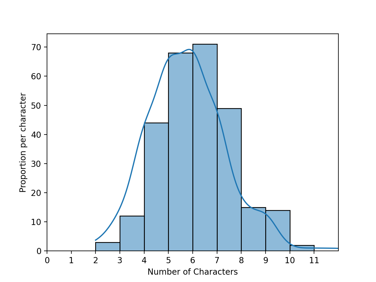
In lecture and Chapter 1 of the textbook, we looked at first names for students taking data science at UC Berkeley as well as the baby names data set from the Social Security Administration. We explored properties such as the lengths of names:
For this program, we will focus on the most common names in a given file, as well the names that make up a fixed fraction of the names. To allow for unit testing, the assignment is broken into the following functions: For example, assuming these functions are in a file, Another example with a file korea_most_pop2019.txt, containing the most popular names in South Korea in 2019, separated by both newlines and spaces:
Notes: you should submit a file with only the standard comments at the top, and these functions. The grading scripts will then import the file for testing and expect the functions to match in name and return values to above:
Learning Objective: to build competency with string and file I/O functionality of core Python.
Available Libraries: Core Python 3.6+ only.
extract_names(file_name, sep = ["\n"]): Returns a list of names. Assumes that the names are separated by the separators listed in sep. The default value is ["\n"] but the possible inputs are 1 or more separators. Your function should remove any empty strings from the list.
count_names(names_lst):
Returns a dictionary of names with values the number of times each name occurs in the input, names_lst.
popular_names(names_dict,num = 3):
Returns a list of the num most popular names as a list of strings. If no value is passed for num, the default value of 3 is used (that is, it returns the 3 most popular names).
percent_captured(names_dict,threshold = 75):
Returns the number of names needed to have at least threshold percent of all the names in the dictionary. If no value is passed for percent, the default value of 75 is used (that is, it returns the number of names needed to have 75 percent (or more) of the total occurrances of names).
p1.py and run on a file containing names that start with 'A', a_names.txt:
gives the output:
lst = p1.extract_names('a_names.txt')
print(f'The list is:\n{lst}')
dict = p1.count_names(lst)
print(f'The dictionary is:\n{dict}')
lstTop = p1.popular_names(dict)
print(f'The top 3 names are: {lstTop}.')
num = p1.percent_captured(dict, threshold = 50)
print(f'The top {num} names make up 50% of the list.')
The list is:
['Alex', 'Andy', 'Amy', 'Alani', 'Alex', 'Ana', 'Angela', 'Ai', 'Asia', 'Alex', 'Anna', 'Ana', 'Asami', 'Andrea', 'Alex', 'Ana', 'Anya', 'Aiko', 'Ana', 'Angela', 'Ai', 'Alexander', 'Alex', 'Ana', 'Andy']
The dictionary is:
{'Alex': 5, 'Andy': 2, 'Amy': 1, 'Alani': 1, 'Ana': 5, 'Angela': 2, 'Ai': 2, 'Asia': 1, 'Anna': 1, 'Asami': 1, 'Andrea': 1, 'Anya': 1, 'Aiko': 1, 'Alexander': 1}
The top 3 names are: ['Alex', 'Ana', 'Andy'].
The top 4 names make up 50% of the list.
gives the output:
lst = p1.extract_names('korea_most_pop2019.txt',sep=["\n"," "])
print(lst)
['Ji-an', 'Ha-yoon', 'Seo-ah', 'Ha-eun', 'Seo-yun', 'Ha-rin', 'Ji-yoo', 'Ji-woo', 'Soo-ah', 'Ji-a', 'Seo-jun', 'Ha-joon', 'Do-yun', 'Eun-woo', 'Si-woo', 'Ji-ho', 'Ye-jun', 'Yu-jun', 'Ju-won', 'Min-jun']
If your file includes code outside of these functions, either comment the code out before submitting or use a main function that is conditionally executed (see Think CS: Section 6.8 for details).
"""
Name:  YOUR NAME
Email: YOUR EMAIL
Resources:  RESOURCES USED
"""

def extract_names(file_name, sep = ["\n"]):
    """
    Opens and reads from file_name, and returns a list of names.

    Keyword arguments:
    sep -- the deliminators for splitting up the data (default ['\n'])
    """

    #Placeholder-- replace with your code
    lst = []
    return lst

def count_names(names_lst):
    """
    Returns a dictionary of names with values the number of times
    each name occurs in the input, names_lst.
    """

    #Placeholder-- replace with your code
    dict = {}
    return dict

def popular_names(names_dict,num = 3):
    """
    Returns a list of the num most popular names as a list of strings.

    Keyword arguments:
    sep -- the number of names to return (default is 3)
    """

    #Placeholder-- replace with your code
    lst = []
    return lst


def percent_captured(names_dict,threshold = 75):
    """
    Returns the number of names needed to have at least threshold percent of
    all the names in the dictionary.

    Keyword arguments:
    threshold -- the percent used for threshold (default 75)
    """

    #Placeholder-- replace with your code
    count = 0
    return count
Program 2: Parking Tickets. Due noon, Thursday, 17 February.
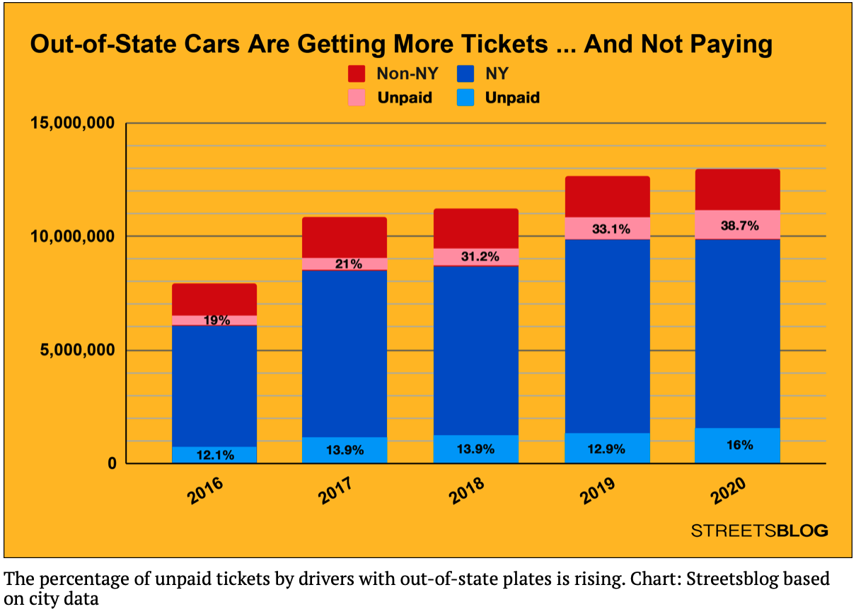
Recent news articles focused on the significantly higher percentage of parking tickets that are unpaid for cars with out-of-state plates:
The data is aggregated across the whole city. Does the same occur when the datasets are focused on individual neighborhoods? To answer that question, as well as what are the most common reasons for tickets, we will use the parking ticket data from OpenData NYC. In Lecture 3, we started data cleaning efforts on the parking ticket data. We will continue the data cleaning efforts for this program, as well as introduce auxiliary files that link the codes stored with a short explanation of the violation. The assignment is broken into the following functions to allow for unit testing:
For example, assuming your functions are in the Looking at the registration types ( And for the Precinct District 19 dataset that contains almost a half million tickets:
Learning Objective: to refresh students' knowledge of Pandas' functionality to manipulate and create columns from formatted data.
Available Libraries: Pandas and core Python 3.6+.
make_df(file_name):
This function takes one input:
The function should open the file file_name: the name of a CSV file containing Parking Ticket Data from OpenData NYC.
file_name as DataFrame, drop all but the columns:
and return the resulting DataFrame.
Summons Number,Plate ID,Registration State,Plate Type,Issue Date,Violation Code,Violation Time,
Violation In Front Of Or Opposite,House Number,Street Name,Vehicle Color
filter_reg(df, keep = ["COM", "PAS"]):
This function takes two inputs:
The function returns the DataFrame with only rows that have df: a DataFrame that
including the Plate Type column.
keep: a list of values for the
Plate Type column.
The default value is ["COM", "PAS"].
Plate Type with a value from the list keep. All rows where the Plate Type column contains a different value are dropped.
add_indicator(reg_state):
This function takes one input:
The function should return reg_state: a string containing the state of registation.
1 when reg_state is in ["NY","NJ","CT"] and 0 otherwise.
find_tickets(df, plate_id):
This function takes two inputs:
returns, as a list, the df: a DataFrame that
including the Plate ID column.
plate_id: a string containing a license plate (combination of letters, numbers and spaces).
Violation Code for all tickets issued to that plate_id. If that plate_id has no tickets in the DataFrame, then an empty list is returned.
make_dict(file_name, skip_rows = 1):
This function takes two inputs:
Make a dictionary from a text file named file_name: a string containing the name of a file.
skip_rows: the number of rows to skip at the beginning of file.
The default value is 1.
file_name, where each line, after those that are skipped, makes a dictionary entry. The key for each entry is the string upto the first comma (',') and the value is the string between the first and second commas. All characters after the second comma on a line are ignored.
p2.py:
will print:
df = p2.make_df('Parking_Violations_Issued_Precinct_19_2021.csv')
print(df)
Note that all the rows are included (451,509) but that only the 11 specified columns are retained in the DataFrame.
        Summons Number Plate ID  ...     Street Name Vehicle Color
0           1474094223  KDT3875  ...            E 75         BLACK
1           1474094600  GTW5034  ...  EAST 70 STREET            BK
2           1474116280  HXM6089  ...         E 72 ST            BK
3           1474116310  HRW4832  ...         E 72 ST           GRY
4           1474143209  JPR6583  ...  EAST 94 STREET         BLACK
...                ...      ...  ...             ...           ...
451504      8954357854  JRF3892  ...         5th Ave            GR
451505      8955665040   199VP4  ...       E 74th St         BLACK
451506      8955665064   196WL7  ...       E 78th St         BLACK
451507      8970451729  CNK4113  ...        York Ave            GY
451508      8998400418   XJWV98  ...        York Ave         WHITE

[451509 rows x 11 columns]Plate Type):
prints many different types of registrations and abbreviations:
print(f"Registration: {df['Plate Type'].unique()}")
print(f"\n10 Most Common:  {df['Plate Type'].value_counts()[:10]}")
The two registration types that are the most common:
Registration: ['PAS' 'SRF' 'OMS' 'COM' '999' 'SPO' 'OMT' 'MOT' 'RGL' 'PHS' 'MED' 'TRC'
 'APP' 'SRN' 'OML' 'ITP' 'CMB' 'ORG' 'AMB' 'DLR' 'IRP' 'TOW' 'MCL' 'CBS'
 'LMB' 'USC' 'CME' 'RGC' 'VAS' 'ORC' 'HIS' 'STG' 'AGR' 'TRA' 'CHC' 'SOS'
 'BOB' 'OMR' 'TRL' 'AGC' 'CSP' 'PSD' 'SPC' 'MCD' 'NLM' 'CMH' 'LMA' 'JCA'
 'SCL' 'HAM' 'AYG' 'NYA' 'OMV']

10 Most Common:  PAS    262875
COM    168827
SRF      2834
APP      2800
OMT      2603
OMS      2464
MED      1433
999      1352
CMB      1208
LMB      1135
Name: Plate Type, dtype: int64count = len(df)
pasCount = len(df[df['Plate Type'] == 'PAS'])
comCount = len(df[df['Plate Type'] == 'COM'])
print(f'{count} different vehicles, {100*(pasCount+comCount)/count} percent are passenger or commercial plates.')
Our function will filter for just passenger and commercial plates:
451509 different vehicles, 95.61315499801776 percent are passenger or commercial plates.
will print:
dff = p2.filter_reg(df)
print(f'The length of the filtered data frame is {len(dff)}.')
By specifying different registration types with the keyword argument, we can filter for other registration (DMV's Registration Types) such as motocycles:
The length of the filtered data frame is 431702.
df2 = p2.filter_reg(df,keep=['MOT','HSM','LMA','LMB'])
print(f'The length of the filtered data frame is {len(df2)}.')The length of the filtered data frame is 2095.df2['NYPlates'] = df2['Registration State'].apply(p2.add_indicator)
print(df2.head()) Summons Number Plate ID ... Vehicle Color NYPlates
3888 8778381423 MD677M ... SILVE 1
5967 1475041184 92BF34 ... BLK 1
6177 1477342850 40TZ78 ... RD 1
6985 8514394770 16UD95 ... BLACK 1
7221 8624098440 77BD79 ... BLACK 1Plate ID and use the dictionary of the violation code to find out what the tickets were for:
print(f'Motorcycles with most tickets:\n {df2["Plate ID"].value_counts()[:5]}')
code_lookup = p2.make_dict('ticket_codes.csv')
ticket_codes = p2.find_tickets(df2,'19UB23')
descrip = [code_lookup[str(t)] for t in ticket_codes]
print(f'The motocycle with plate 19UB23 got the following tickets: {descrip}')Motorcycles with most tickets:
19UB23 14
80BD05 10
38SV33 9
66TZ74 8
70TW50 8
Name: Plate ID, dtype: int64
The motocycle with plate 19UB23 got the following tickets: ['NO PARKING-STREET CLEANING', 'REG. STICKER-EXPIRED/MISSING', 'REG. STICKER-EXPIRED/MISSING', 'INSP. STICKER-EXPIRED/MISSING', 'REG. STICKER-EXPIRED/MISSING', 'REG. STICKER-EXPIRED/MISSING', 'REG. STICKER-EXPIRED/MISSING', 'REG. STICKER-EXPIRED/MISSING', 'INSP. STICKER-EXPIRED/MISSING', 'REG. STICKER-EXPIRED/MISSING', 'REG. STICKER-EXPIRED/MISSING', 'REG. STICKER-EXPIRED/MISSING', 'REG. STICKER-EXPIRED/MISSING', 'REG. STICKER-EXPIRED/MISSING']Note: you should submit a file with only the standard comments at the top, this function, and any helper functions you have written. The grading scripts will then import the file for testing. If your file includes code outside of functions, either comment the code out before submitting or use a main function that is conditionally executed (see Think CS: Section 6.8 for details).
Hints:- Parking ticket data can be found at: NYC OpenData.
- Some datasets for testing:
- parking_test_100.csv: A truncated file for testing-- first 100 rows of the 2021 UES parking tickets (described below).
- Parking_Violations_Issued_Precinct_19_2021.csv: ~450,000 line file of parking violations issues in 2021 for the Upper East Side (District 19)
- Parking ticket violation codes (summary of codes & fines) are the basis for the dictionary.
- ticket_codes.csv from OpenData NYC.
- You may get a warning such as:
sys:1: DtypeWarning: Columns (39) have mixed types.Specify dtype option on import or set low_memory=False.when reading in the parking ticket data. Pandas tries to infer the data type (dtype) of the columns from the values. Since some columns are a mixture of numeric and character types this can be difficult. If the file is read in withpd.read_csv(file_name, low_memory=False), the entire column is read in and used to determine type.
Program 3: Restaurant Rankings. Due noon, Thursday, 24 February.
The NYC Department of Health & Mental Health regularly inspects restaurants and releases the results:
These results are also available in CSV files at
https://data.cityofnewyork.us/Health/DOHMH-New-York-City-Restaurant-Inspection-Results/43nn-pn8j. This programming assignment focuses on predicting letter grades for restaurants, yet to be graded, as well computing summary statistics by neighborhood.
The assignment is broken into the following functions to allow for unit testing:
For example, assuming your functions are in the Using the We can use the numeric grade to compute the averages for neighborhoods for both provided and predicted scores:
To make it easier to find scores for neighborhoods we combine with the NTA table:
Hints:
Learning Objective: students can successfully filter formatted data using standard Pandas operations for selecting and joining data.
Available Libraries: Pandas and core Python 3.6+.
make_insp_df(file_name):
This function takes one input:
The function should open the file file_name: the name of a CSV file containing Restaurant Inspection Data from OpenData NYC.
file_name as DataFrame, keeping only the columns:
If the 'CAMIS', 'DBA', 'BORO', 'BUILDING', 'STREET', 'ZIPCODE', 'SCORE', 'GRADE', 'NTA'SCORE is null for a row, that row should be dropped. The resulting DataFrame is returned.
predict_grade(num_violations):
This function takes one input:
The function should then return the letter grade that corresponds to the number of violation points num_violations: the number of violations points.
num_violations:
(from NYC Department of Health
Restaurant Grading).
grade2num(grade):
This function takes one input:
and returns the grade on a 4.0 scale for grade: a letter grade or null value.
grade = 'A', 'B', or 'C' (i.e. 4.0, 3.0, or 2.0, respectively). If grade is None or some other value,
return None.
make_nta_df(file_name):
This function takes one input:
The function should open the file file_name: the name of a CSV file containing neighborhood tabulation areas (nynta.csv).
file_name as DataFrame, returns a DataFrame
containing only the columns, NTACode and NTAName.
compute_ave_grade(df,col):
This function takes two inputs:
This function returns a DataFrame and returns a DataFrame with two columns, the df: a DataFrame containing Parking Ticket Data from OpenData NYC.
col: the name of a numeric-valued col in the DataFrame.
NTACode and the average of col for each NTA.
neighborhood_grades(ave_df,nta_df):
This function takes two inputs:
This function returns a DataFrame and returns a DataFrame with the neighborhood codes and names ('NTAName') and the columns from ave_df
This function takes a df containing NTACode and the nta_df containing
NTA and returns the joins on these two columns, dropping both before returning.
ave_df: a DataFrame with containing the column 'NTACode'
nta_df: a DataFrame with two columns, 'NTACode' and 'NTAName'.
p3.py:
will print:
df = p3.make_insp_df('restaurants1Aug21.csv')
print(df)
Note that all the rows are included (243) but that only the 9 specified columns are retained in the DataFrame. Several rows have null entries for CAMIS DBA BORO ... SCORE GRADE NTA
0 41178124 CAFE 57 Manhattan ... 4.0 A MN15
1 50111450 CASTLE CHICKEN Bronx ... 41.0 N BX29
2 40699339 NICK GARDEN COFFEE SHOP Bronx ... 31.0 NaN BX05
3 41181395 DUNKIN' Brooklyn ... 10.0 A BK25
4 50052976 ZON BAKERY & CAFE Manhattan ... 72.0 NaN MN36
.. ... ... ... ... ... ... ...
240 50052976 ZON BAKERY & CAFE Manhattan ... 72.0 NaN MN36
241 41525768 THE WEST CAFE Brooklyn ... 10.0 A BK73
242 50111132 BUONASERA RESTAURANT PIZZA Brooklyn ... 16.0 N BK30
243 40399672 BAGELS & CREAM CAFE Queens ... 12.0 A QN06
244 50104259 ROYAL COFFEE SHOP Staten Island ... 69.0 N SI22
[243 rows x 9 columns]GRADE (e.g. row 2, 4, and 240) while others have letter grades (such as 'N') that are not on the list of possible grades.
SCORE to compute the likely grade for each inspection, as both a letter and its equivalent on a 4.0 grading scale, yields:
prints many the predicted grade and equivalent numeric grade on the 4.0 scale:
df['NUM'] = df['GRADE'].apply(p3.grade2num)
df['PREDICTED'] = df['SCORE'].apply(p3.predict_grade)
df['PRE NUM'] = df['PREDICTED'].apply(p3.grade2num)
print(df[ ['DBA','SCORE','GRADE','NUM','PREDICTED','PRE NUM'] ]) DBA SCORE GRADE NUM PREDICTED PRE NUM
0 CAFE 57 4.0 A 4.0 A 4.0
1 CASTLE CHICKEN 41.0 N NaN C 2.0
2 NICK GARDEN COFFEE SHOP 31.0 NaN NaN C 2.0
3 DUNKIN' 10.0 A 4.0 A 4.0
4 ZON BAKERY & CAFE 72.0 NaN NaN C 2.0
.. ... ... ... ... ... ...
240 ZON BAKERY & CAFE 72.0 NaN NaN C 2.0
241 THE WEST CAFE 10.0 A 4.0 A 4.0
242 BUONASERA RESTAURANT PIZZA 16.0 N NaN B 3.0
243 BAGELS & CREAM CAFE 12.0 A 4.0 A 4.0
244 ROYAL COFFEE SHOP 69.0 N NaN C 2.0
[243 rows x 6 columns]
The first couple of rows are:
actual_scores = p3.compute_ave_grade(df,'NUM')
predicted_scores = p3.compute_ave_grade(df,'PRE NUM')
scores = actual_scores.join(predicted_scores, on='NTA')
print(scores.head()) NUM PRE NUM
NTA
BK09 4.0 4.000000
BK17 4.0 4.000000
BK25 4.0 4.000000
BK26 NaN 2.000000
BK28 4.0 3.250000
The first couple of rows are:
nta_df = p3.make_nta_df('nynta.csv')
scores_with_nbhd_names = p3.neighborhood_grades(scores,nta_df)
print(scores_with_nbhd_names.head())
Our predicted scores are the same but almost always decrease when we include the predicted grades from the scores reported.
    NUM   PRE NUM                                         NTAName
0   4.0  4.000000                    Brooklyn Heights-Cobble Hill
1   4.0  4.000000  Sheepshead Bay-Gerritsen Beach-Manhattan Beach
2   4.0  4.000000                                       Homecrest
3   NaN  2.000000                                       Gravesend
4   4.0  3.250000                                Bensonhurst West
sys:1: DtypeWarning: Columns (39) have mixed types.Specify dtype option on import or set low_memory=False.
when reading in the parking ticket data. Pandas tries to infer the data type (dtype) of the columns from the values. Since some columns are a mixture of numeric and character types this can be difficult. If the file is read in with pd.read_csv(file_name, low_memory=False), the entire column is read in and used to determine type.
numeric_only = True.
More to come...
Project
A final project is optional for this course.
Projects should synthesize the skills acquired in the course to analyze and visualize data on a topic of your choosing. It is your chance to demonstrate what you have learned, your creativity, and a project that you are passionate about. The intended audience for your project is your classmates as well as tech recruiters and potential employers.
The grade for the project is a combination of grades earned on the milestones (e.g. deadlines during the semester to keep the projects on track) and the overall submitted program. If you choose not to complete the project, your final exam grade will replace its portion of the overall grade.
Milestones
The project is broken down into smaller pieces that must be submitted by the deadlines below. For details of each milestone, see the links. The project is worth 20% of the final grade. The point breakdown is listed as well as the submission windows and deadlines. All components of the project are submitted via Gradescope unless other noted.
| Deadline: | Deliverables: | Points: | Submission Window Opens: |
|---|---|---|---|
| Monday, 28 February, noon | Opt-In | 14 February | |
| Monday, 7 March, noon | Proposal | 50 | 1 March |
| Monday, 4 April, noon | Interim Check-In | 25 | 14 March |
| Monday, 25 April, noon | Complete Project & Website | 100 | 5 April |
| Monday, 9 May, noon | Presentation Slides | 25 | 14 April |
| Total Points: | 200 | ||
Project Opt-In
Review the following FAQs before filling out the Project Opt-In form (available on Gradescope on 14 February).- Is the final project mandatory?
No, the final project is optional for this course. - Will the project be difficult?
Expect the project to be time consuming because we will hold you to a high standard. However, in turn, we hope that this will produce a high quality project that you could proudly add to your coding portfolio, to showcase when seeking internships and full-time jobs. - What counts as "opting in" to the project?
That's easy. Your response to this Gradescope assignment counts as your "opt in". If you respond "No" or do not submit this assignment before the deadline due date, we will count you as having "opted out". - What happens after I "opt in"?
If you "opt in", we will continue to send you information on completing the next steps for the final project via Gradescope. If you "opt out", you will no longer receive follow up assignments for the project. - Does "opting in" place me under obligation to complete the project?
Yes and no. We would like you to seriously consider your availability before making this commitment. Likewise, we would like to focus our time to help those who are serious about doing this project. That being said, if you decide midway through the process that you no longer have the time nor capacity to complete the project, no harm no foul, your final written exam will once again be weighted 40% of your cumulative grade (see more in the question below). - How does the final project factor into my final grade?
If you choose to do the project, your Written Exam will be worth 20% of your overall course grade:- Optional Project: 20%
- Final Exam - Written Exam: 20%
- Final Exam - Coding Exam: 20%
- Final Exam - Written Exam: 40%
- Final Exam - Coding Exam: 20%
Project Proposal
The window for submitting proposals opens 1 March. If you would like feedback and the opportunity to resubmit for a higher grade, submit early in the window. Feel free to re-submit as many times as you like, up until the assignment deadline. The instructing team will work hard to give feedback on your submission as quickly as possible, and we will grade them in the order they were received.
The proposal is split into the following sections:
- Overview: (10 Points)
Think of the overview section as the equivalent of an abstract in a research paper or an elevator pitch for the project. The following questions will help you frame your thoughts if you ever have to succinctly describe your project in an interview:- Title: should capture the topic/theme of your project.
- Objective: In 1 to 2 sentences, succinctly describe what you are hoping to accomplish in this project in simple, non technical English.
- Importance: In 1 to 2 sentences, describe why this project has personal significance to you.
- Originality: In 1 to 2 sentences, describe why you believe this project idea is unique and original.
- Background Research: (10 Points)
In this section, please prove to us that you have already done research in the project you are proposing by answering the questions below.- Key Term Definitions: What are some terms specific to your project that someone else might not know? List and define these terms here.
- Existing Solutions: What are some existing solutions (if any) that are already available for your problem. What are the drawbacks to these solutions?
- Data: (10 points)
In order to write a successful proposal, you must already have obtained the data and done basic exploratory analysis on it, enough so that you feel confident you have enough data to answer the questions you wish to explore. We cannot stress this enough: You must use NYC specific data that is publicly available. If your data does not fit this criteria, your proposal will be rejected.The following questions will guide you through some criteria you should be using to assess if the data you have is enough for a successful project.
- Data Source: Include a list of your planned data source(s), complete with URL(s) for downloading. All data must be NYC specific and must be publicly available.
- Data Volume: How many columns in your dataset? How many rows? If you are joining multiple datasets together, please tell us how many rows and columns remain after the data has been merged into a single dataset.
- Data Richness: What type of data is in your dataset? You don't need to describe every column. A generalized overview is fine. (e.g. "My data contains 311 complaint types, the date the complaints are created and closed, as well as a description of the complaint"). If you found a data dictionary, feel free to link us to that as well.
- The Predictive Model: (10 Points)
A strong data science project should demonstrate your knowledge of predictive modeling. We will be covering models extensively in the latter half of the course. At this stage of the proposal writing, we will not have covered all the modeling techniques yet, so it's okay to be a bit vague here.Hint: Look ahead in the textbook at the chapters on "Linear Modeling" and "Multiple Linear Modeling" for the running examples of models.
- The Predicted (Y): Which column in the dataset are you interested in predicting?
- The Predictors (X's): Which column(s) in the dataset will be used to predict the column listed above?
- Python Dependencies: What Python libraries and dependencies will you be using?
- Security and Privacy Considerations: Will you be working with personal identifiable information (PII)? Can your model be mis-used for evil, not good? If so, how do you plan to mitigate that?
- The Visualization: (10 Points)
A key part of making a great data science portfolio are the visualizations. This is a quick and elegant way of showcasing your work during the job hunting process, even to a non-technical audience.Thus, a major part of this final project will center around making the following three types of visualizations with the data you choose. If your data cannot support all three types of visualizations, then please, reconsider choosing another dataset.
- Summary Statistics Plots: Write out in detail at least 3 types of summary statistics graphs you plan to make with your data (e.g. "I plan to make a histogram using the column X").
- Map Graphs: Write out in detail how you plan to make at least 1 map data visualization using your data (e.g. "I plan to create a choropleth map to visualize the volume of 311 service requests in NYC in 2021").
- Model Performance Plots: At the time of writing this proposal, we would not have covered how to visualize model accuracy yet. So, no worries if this part is still confusing to you. Give it your best shot on explaining what kind of visualization you think will best showcase that your model is "successful" and "accurate".
More to come...