Program 8, CSci 39542: Data Science, Hunter College

Program 8: Yellow Taxi Data
CSci 39542: Introduction to Data Science
Department of Computer Science
Hunter College, City University of New York
Spring 2022

Program Description

Program 8: Yellow Taxi Data. Due noon, Thursday, 31 March.
Learning Objective: give students practice on implementing model from start to finish and to strengthen understanding of model drift.
Available Libraries: pandas, datetime, sklearn, and core Python 3.6+.
Data Sources: Yellow Taxi Trip Data from OpenData NYC.
Sample Datasets: taxi_new_years_day_2020.csv, taxi_4July2020.csv, and taxi_jfk_june2020.csv.

This program as well as the following program, Program 9, are tailored to the NYC OpenData Yellow Taxi Trip Data and follow a standard strategy for data cleaning and model building of:

Read in datasets, merging and cleaning as needed.
Impute missing values (we will use median for the numeric values).
Transform features to polynomial (we will restrict to quadratic).
Split our dataset into training and testing sets.
Fit a model, or multiple models, to the training dataset.
Validate the models using the testing dataset.

This program will focus on building a linear regression model on the numerical features of our dataset to predict tip percentages. In Program 9, we also encode and impute categorical data features to build a model to predict which taxi trips paid tolls.

The function specifications are:

import_data(file_name) -> pd.DataFrame: This function takes as one input parameter:
- file_name: the name of a CSV file containing Yellow Taxi Trip Data from OpenData NYC.
The data in the file is read into a DataFrame, any rows with non-positive total_amount are dropped. The resulting DataFrame is returned.
add_tip_time_features(df) -> pd.DataFrame: This function takes one input:
- df: a DataFrame containing Yellow Taxi Trip Data from OpenData NYC.
The function computes 3 new columns:
- percent_tip: which is 100*tip_amount/(total_amount-tip_amount)
- duration: the time the trip took in seconds.
- dayofweek: the day of the week that the trip started, represented as 0 for Monday, 1 for Tuesday, ... 6 for Sunday.
The original DataFrame with these additional three columns is returned.
impute_numeric_cols(df, x_num_cols) -> pd.DataFrame: This function takes two inputs:
- df: a DataFrame containing Yellow Taxi Trip Data from OpenData NYC.
- x_num_cols: a list of numerical columns in df.
Missing data in the columns x_num_cols are replaced with the median of the column. Returns a DataFrame containing only the imputed numerical columns from input df.
transform_numeric_cols(df_num, degree_num=2) -> np.ndarray: This function takes two inputs:
- df_num: a DataFrame of numeric columns with no null values.
- degree_num: the degree used for the polynomial encoding.
An object of sklearn.preprocessing.PolynomialFeatures is instantiated with inputs degree=degree_num and include_bias=False (as discussed in lecture and textbook, we will not include bias when fitting these models). The model is than fitted (using fit_transform) to the numeric columns, df_num, and the resulting array is returned. (See Chapter 20.2.2 for an example).
fit_linear_regression(x_train, y_train) This function takes two inputs:
- x_train: an array of numeric columns with no null values.
- y_train: an array of numeric columns with no null values.
Fits a linear model to x_train and y_train, using sklearn.linear_model.LinearRegression (see lecture & textbook for details on setting up the model). The function returns the intercept (intercept_), the model coefficients (coef_), and model object that you constructed.
predict_using_trained_model(mod, x, y): This function takes three inputs:
- mod: a trained model for the data.
- x: an array or DataFrame of numeric columns with no null values.
- y: an array or DataFrame of numeric columns with no null values.
Computes and returns the mean squared error and r2 score between the values predicted by the model (mod on x) and the actual values (y). Note that sklearn.metrics contains two functions that may be of use: mean_squared_error and r2_score.

For example, the file, taxi_jfk_june2020.csv, contains all taxi trips, starting from JFK in June 2020 Yellow Taxi Trip Data (about 9,500 entries) with the first lines are:

VendorID,tpep_pickup_datetime,tpep_dropoff_datetime,passenger_count,trip_distance,RatecodeID,store_and_fwd_flag,PULocationID,DOLocationID,payment_type,fare_amount,extra,mta_tax,tip_amount,tolls_amount,improvement_surcharge,total_amount,congestion_surcharge
2,06/01/2020 12:00:31 AM,06/01/2020 12:31:43 AM,1,12.59,1,N,132,189,2,37,0.5,0.5,0,0,0.3,38.3,0
2,06/01/2020 12:05:23 AM,06/01/2020 12:29:05 AM,1,15.8,1,N,132,255,1,42,0.5,0.5,8.66,0,0.3,51.96,0
2,06/01/2020 12:06:27 AM,06/01/2020 12:36:26 AM,1,18.19,2,N,132,142,1,52,0,0.5,10,0,0.3,65.3,2.5
2,06/01/2020 12:08:48 AM,06/01/2020 12:40:48 AM,2,19,2,N,132,113,1,52,0,0.5,13.82,0,0.3,69.12,2.5
2,06/01/2020 12:13:46 AM,06/01/2020 12:25:29 AM,1,7.21,1,N,132,134,2,21,0.5,0.5,0,0,0.3,22.3,0

Then our first functions:

df = import_data('taxi_jfk_june2020.csv')
df = add_tip_time_features(df)
print(df[ ['trip_distance','duration','dayofweek','total_amount','percent_tip'] ].head() )

prints:

   trip_distance  duration  dayofweek  total_amount  percent_tip
0          12.59    1872.0          0         38.30     0.000000
1          15.80    1422.0          0         51.96    20.000000
2          18.19    1799.0          0         65.30    18.083183
3          19.00    1920.0          0         69.12    24.990958
4           7.21     703.0          0         22.30     0.000000

We can impute the missing data in numerical columns with their median value. For example:

print(df[ ['passenger_count','trip_distance'] ].head(10) )
df['passenger_count'] = impute_numeric_cols(df,['passenger_count'])
print( df[ ['passenger_count','trip_distance'] ].head(10) )

shows the passenger_count the results of impute_numeric_cols:

   passenger_count  trip_distance
0              1.0          12.59
1              1.0          15.80
2              1.0          18.19
3              2.0          19.00
4              1.0           7.21
5              1.0           6.50
6              2.0          13.90
7              NaN           0.00
8              NaN           0.00
9              NaN           0.00
   passenger_count  trip_distance
0              1.0          12.59
1              1.0          15.80
2              1.0          18.19
3              2.0          19.00
4              1.0           7.21
5              1.0           6.50
6              2.0          13.90
7              1.0           0.00
8              1.0           0.00
9              1.0           0.00

The running example in the textbook focuses on predicting restaurant tips. A highly correlated feature with tips for restaurant meals is the total bill. Let's look at the taxi data set to see if a similar correlation is suggested for tips on yellow taxi trips:

#Explore some data:
import matplotlib.pyplot as plt
import seaborn as sns
sns.set_theme(color_codes=True)

sns.lmplot(x="total_amount", y="percent_tip", data=df)
tot_r = df['total_amount'].corr(df['percent_tip'])
plt.title(f'Taxi Trips from JFK, June 2020 with r = {tot_r:.2f}')
plt.tight_layout()  #for nicer margins
plt.show()
sns.lmplot(x="trip_distance", y="percent_tip", data=df)
dist_r = df['trip_distance'].corr(df['percent_tip'])
plt.title(f'Taxi Trips from JFK, June 2020 with r = {dist_r:.2f}')
plt.tight_layout()  #for nicer margins
plt.show()

The resulting images:

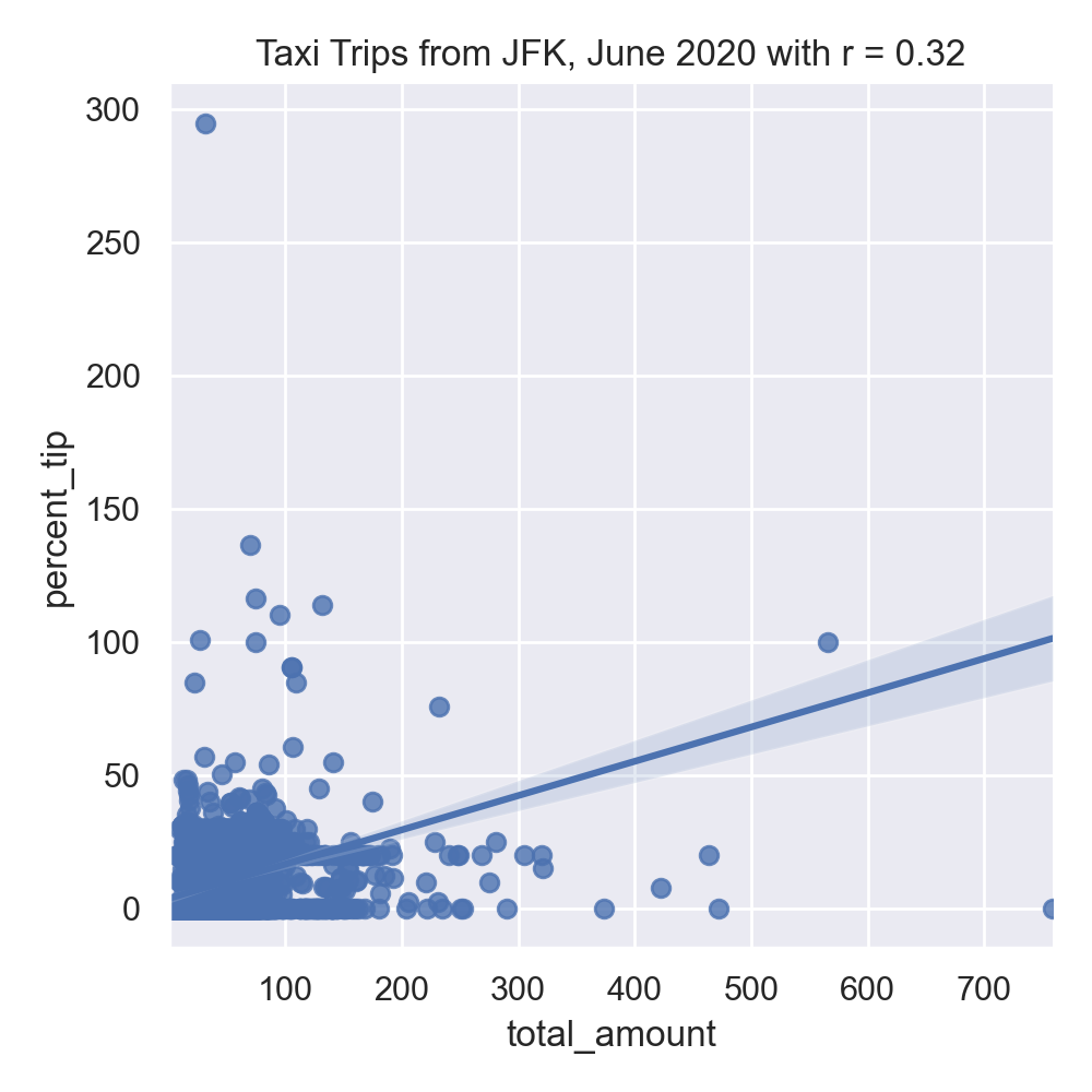
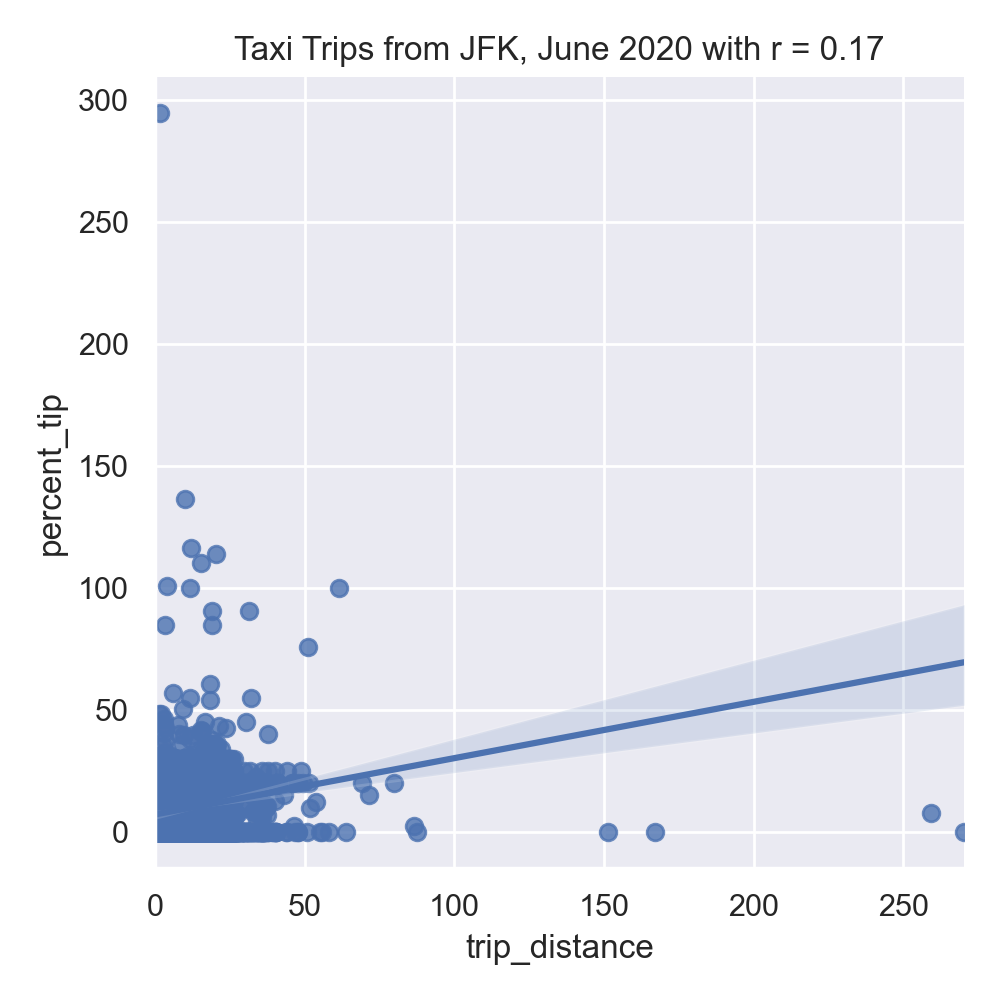
Neither total amount or distance of the trip are strongly correlated, suggesting a linear regression model with a single input will not make a good predictor. Let's build a more complicated model that uses multiple inputs, including the numerical columns:

num_cols = ['passenger_count','trip_distance','RatecodeID','PULocationID','DOLocationID','payment_type','fare_amount','extra','mta_tax','tip_amount','tolls_amount','improvement_surcharge','total_amount','congestion_surcharge','duration','dayofweek']
df_imputed = impute_numeric_cols(df,num_cols)
df_x = df_imputed
y = df['percent_tip']

With the missing numeric data imputed, we can fit the model on training sets (of size 25%):

from sklearn.model_selection import train_test_split
print('For numeric columns, training on 25% of data:')
x_train,x_test,y_train,y_test = train_test_split(df_x,y)
intercept, coeffs, mod = fit_linear_regression(x_train,y_train)
print(f'intercept = {intercept} and coefficients = {coeffs}')
tr_err,tr_r2 = predict_using_trained_model(mod, x_train,y_train)
print(f'training:  RMSE = {tr_err} and r2 = {tr_r2}.')
test_err,test_r2 = predict_using_trained_model(mod, x_test,y_test)
print(f'testing:  RMSE = {test_err} and r2 = {test_r2}.')

the resulting model does a reasonable both with the training and testing data sets that we used to validate the model:

For numeric columns, training on 25% of data:
intercept = 34.128603724366776 and coefficients = [-4.51251635e-02  1.42762012e-01 -2.13115277e-01  5.25968158e-15
 -2.55903361e-03 -6.90080569e+00  4.14314789e-02  1.10260155e-02
 -3.02379090e+00  1.29921229e+00  1.10123016e-01 -4.40906348e+01
 -1.81824685e-01  5.12722540e-02 -3.16853791e-05  1.08447199e-02]
training:  RMSE = 34.01017686662997 and r2 = 0.7350167925786109.
testing:  RMSE = 23.9974484390634 and r2 = 0.798760914470428.

We can use the model for other yellow taxi data sets to see how well our model does:

print(f'Prediction for 4 July data:')
df_july = pd.read_csv('taxi_4July2020.csv').head()
df_july = add_tip_time_features(df_july)
df_j_imp = impute_numeric_cols(df_july,num_cols)
df_x = df_imputed
y = df_july['percent_tip']
df_july_imp = impute_numeric_cols(df_july,num_cols)
july_err,july_r2 = predict_using_trained_model(mod, df_july_imp,df_july['percent_tip'])
print(f'training:  RMSE = {tr_err} and r2 = {tr_r2}.')

The root mean squared error is higher, but still a reasonable fit:

Prediction for 4 July data:
training:  RMSE = 34.01017686662997 and r2 = 0.7350167925786109.

Do we need 25% of the data for training? Let's try with just 10% of the data and see how well the model does on the training and testing data:

print('For numeric columns, training on 10% of data:')
df_x = df_imputed
y = df['percent_tip']
x_train,x_test,y_train,y_test = train_test_split(df_x,y,test_size=0.1,random_state=17)
intercept, coeffs, mod = fit_linear_regression(x_train,y_train)
print(f'intercept = {intercept} and coefficients = {coeffs}')
tr_err,tr_r2 = predict_using_trained_model(mod, x_train,y_train)
print(f'training:  RMSE = {tr_err} and r2 = {tr_r2}.')
test_err,test_r2 = predict_using_trained_model(mod, x_test,y_test)
print(f'testing:  RMSE = {test_err} and r2 = {test_r2}.')

For numeric columns, training on 10% of data:
intercept = 31.93944365469102 and coefficients = [-6.96532365e-02  1.53416173e-01 -1.75092738e-01  4.35768088e-12
 -2.11111185e-03 -6.89816662e+00 -2.41541506e-02  3.72953218e-02
 -3.24270162e+00  1.26217702e+00  2.79494331e-02 -3.67595994e+01
 -1.22350450e-01 -9.82610653e-02 -2.68681888e-05  1.17100065e-02]
training:  RMSE = 31.839870447532608 and r2 = 0.7460779638992571.
testing:  RMSE = 27.58958147548388 and r2 = 0.7913497106610776.

Lastly, we can use quadratic features to build a model:

print('For transformed columns, training on 25% of data:')
df_transformed = transform_numeric_cols(df_imputed)
df_x = df_transformed
x_train,x_test,y_train,y_test = train_test_split(df_x,y)
int_poly, co_poly, mod_poly = fit_linear_regression(x_train,y_train)
print(f'intercept = {int_poly} and coefficients = {co_poly}')
tr_err,tr_r2 = predict_using_trained_model(mod_poly, x_train,y_train)
print(f'training:  RMSE = {tr_err} and r2 = {tr_r2}.')
test_err,test_r2 = predict_using_trained_model(mod_poly, x_test,y_test)
print(f'testing:  RMSE = {test_err} and r2 = {test_r2}.')

the resulting model produces the following parameters and does very well with the training data, but not as well on validation:

testing:  RMSE = 27.58958147548388 and r2 = 0.7913497106610776.
For transformed columns, training on 25% of data:
intercept = 98.72874163717195 and coefficients = [ 2.10419587e-05 -7.33813212e-05  3.36448376e-05 -1.14982704e-03
  3.21888112e-07 -1.44329284e-05 -8.69336745e-04  1.66712369e-04
  2.81695737e-04 -1.08879523e-03  3.41908316e-04  2.12645367e-04
 -1.14415611e-02 -1.90864671e-04 -3.59725562e-05 -1.35384327e-07
  3.16192056e-05 -9.70729528e-03  4.68643310e-02  6.01985117e-03
 -3.18255958e-03  1.30289584e-04 -2.68086479e-01 -3.84924504e-02
 -1.65688146e-02  1.50481295e+00 -5.70407301e-02 -2.27108373e-02
  2.44141763e-02  2.50939438e-02 -1.76656859e-02  2.59647998e-05
 -8.80232044e-04 -1.68208742e-03  4.63169427e-02  4.20433722e-03
  1.43176776e-04  1.06253564e-01 -6.34687088e-03 -5.11306022e-03
 -4.48735254e-01 -1.76742277e-02 -2.67139991e-02 -1.77037894e+00
  4.89418246e-03  6.67734938e-02  2.61976357e-05  5.54436646e-03
  1.98243118e-01 -1.51783343e-01  1.30845509e-03 -3.03937419e-01
 -2.56107583e-01  6.41789127e-03  2.86357901e-01 -3.85596590e-01
 -3.39876707e-01  5.92648639e+01  2.73192850e-01 -2.66978945e-01
 -8.89359192e-05 -6.07624881e-02  2.58565114e-11 -1.84421817e-03
 -1.14789591e-01  2.19810468e-02  3.71806539e-02 -1.43718154e-01
  4.51344132e-02  2.80868768e-02 -1.51028036e+00 -2.52000297e-02
 -4.74896197e-03 -6.65332251e-06  4.16021836e-03  6.31572545e-08
  2.15564627e-03  2.64693081e-04  2.21420140e-05  3.08987702e-02
  6.24975144e-04  2.75875164e-04  7.32510247e-01 -1.97699408e-04
 -9.16773789e-04 -1.59614030e-06 -2.89070057e-04  1.24237417e+00
 -1.54267635e-01 -2.27724946e-01  5.13635975e+00  3.41927378e-04
 -3.14913649e-01 -2.31439213e-02  3.06565666e-01 -6.16213488e-01
 -1.47606798e-04 -8.65390190e-02  3.68778339e-02  1.26272255e-01
  4.81095283e-01  1.45582565e-01  1.27227451e-01 -7.45844272e-02
 -1.05134981e-01 -4.77707890e-01  1.19878534e-04 -1.60477785e-02
  8.79743756e-02 -3.46596353e+00  1.55694466e-01  1.62418563e-01
 -2.61367204e-01 -1.59647359e-01 -3.77665930e-01  1.09330543e-04
  1.09208554e-02 -5.44386948e-04  6.14354603e-01  4.03678198e-01
 -2.39788549e-02 -3.80000807e-01  1.60567166e+00  5.47130715e-05
 -7.00781561e-01  1.16678588e-01  1.72987001e-01  1.02578238e-04
 -1.81873085e-01 -5.69410563e-01  6.15174164e-05 -5.18682465e-02
  8.35896110e-02  6.38338090e-05 -1.52328411e-01 -4.96025702e-01
  1.11070132e-04 -3.21976800e-02 -3.43245537e-03 -3.59795585e-01
 -1.07930916e-05  4.00086335e-03 -4.81844771e-01  6.89662685e-02
  4.69985663e-01 -1.22753069e-04  1.91297859e-02 -8.99424477e-05
  2.04662228e-04  6.33667804e-02  5.53689326e-09  1.30022472e-05
  5.53118040e-03]
training:  RMSE = 13.088491006521934 and r2 = 0.8967712162338656.
testing:  RMSE = 84.80328619938028 and r2 = 0.31582057991135126.

Program 8: Yellow Taxi Data CSci 39542: Introduction to Data Science Department of Computer Science Hunter College, City University of New York Spring 2022

Program Description

Program 8: Yellow Taxi Data
CSci 39542: Introduction to Data Science
Department of Computer Science
Hunter College, City University of New York
Spring 2022