Today's lab will focus on accessing formatted data using Pandas and Unix shell scripts.

Software tools needed: web browser and Python IDLE programming environment with the Pandas package installed.

Using Python, Gradescope, and Blackboard

See Lab 1 for details on using Python, Gradescope, and Blackboard.

Pandas & Reading Data

To make reading files easier, we will use the Pandas library that lets you read in structured data files very efficiently. Pandas, Python Data Analysis Library, is an elegant, open-source package for extracting, manipulating, and analyzing data, especially those stored in 2D arrays (like spreadsheets). It incorporates most of the Python constructs and libraries that we have seen thus far.

(Pandas is installed on all the lab machines. If you are using your own machine, see the directions at the end of Lab 1 for installing packages for Python.)

In Pandas, the basic structure is a DataFrame which stored data in rectangular grids. Let's use this to visualize the change in New York City's population. First, start your file with an import statements for pyplot and pandas:

import matplotlib.pyplot as plt
import pandas as pd
We used matplotlib in the Lab 3 and Lab 4 for plotting. The as plt allows us to use the plotting commands without having to write matplotlib.pyplot everytime, instead we just write plt. Similarly, The as pd allows us to use pandas commands without writing out pandas everytime-- we just write pd.

Next, save the NYC historical population data to the same directory as your program. This is a "comma separated values" file-- which is a plain text file containging spreadsheet data, with commas separating the different columns (thus, the name). Here's the first 10 lines of the file:

Source:  https://en.wikipedia.org/wiki/Demographics_of_New_York_City,,,,,,
* All population figures are consistent with present-day boundaries.,,,,,,
First census after the consolidation of the five boroughs,,,,,,
,,,,,,
,,,,,,
Year,Manhattan,Brooklyn,Queens,Bronx,Staten Island,Total
1698,4937,2017,,,727,7681
1771,21863,3623,,,2847,28423
1790,33131,4549,6159,1781,3827,49447
1800,60515,5740,6642,1755,4563,79215
Note that it has 5 extra lines at the top before the column names occur. The pandas function for reading in CSV files is read_csv(). It has an option to skip rows which we will use here:
pop = pd.read_csv('nycHistPop.csv',skiprows=5)

Before going on, let's print out the variable pop. pop is a dataframe, described in the reading above:

print(pop)
The last line of our first pandas program is:
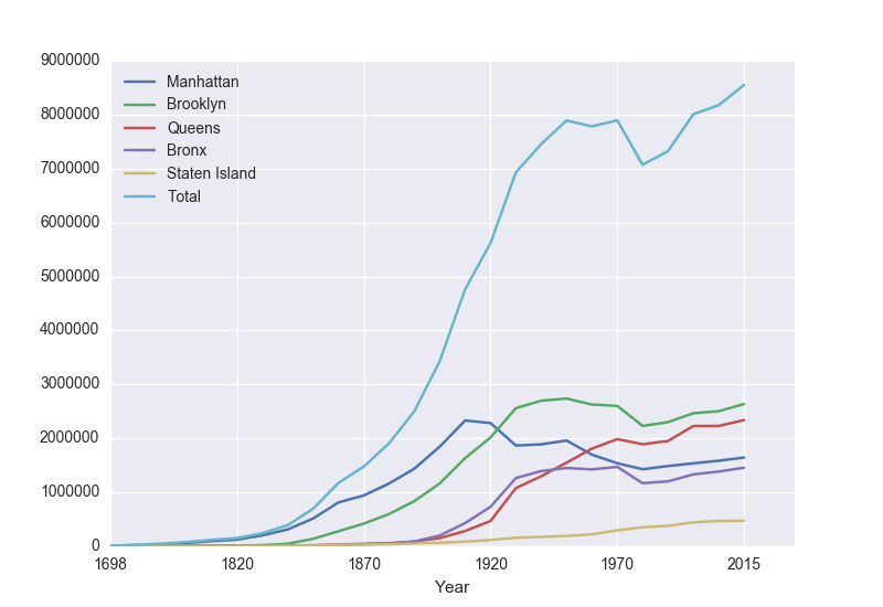
pop.plot(x="Year")
which makes a graphical display of all of the data series in the variable pop with the series corresponding to the column "Year" as the x-axis. Your output should look something like:

To recap: our program is:


import matplotlib.pyplot as plt

import pandas as pd
pop = pd.read_csv('nycHistPop.csv',skiprows=5)
pop.plot(x="Year")

plt.show()

which did the following: There are useful built-in statistics functions for the dataframes in pandas. For example, if you would like to know the maximum value for the series "Bronx", you apply the max() function to that series:
print("The largest number living in the Bronx is", pop["Bronx"].max()) 
Similarly the average (mean) population for Queens can be computed:
print("The average number living in the Queens is", pop["Queens"].mean()) 

Challenges

Manipulating Columns

Each column in the original spreadsheet is a column, or series. We can look at the column for the Bronx with:

    print(pop['Bronx'])
How would you look at the one for Brooklyn?

A nice thing about series is that you can do basic arithmetic with them. For example,

    print(pop['Bronx']*2)
prints out double the values in the column.

You can also use multiple columns in a calculation:

    print(pop['Bronx']/pop['Total'])
prints out the fraction of the total population that lives in the Bronx.

We can save that series by creating a new column for it:

    pop['Fraction'] = pop['Bronx']/pop['Total']
and then can use it to create a new graph:
    pop.plot(x = 'Year', y = 'Fraction')
We can save it to a file, by storing the current figure (via "get current figure" or gcf() function and then saving it:
    fig = plt.gcf()
    fig.savefig('fractionBX.png')
shown in the following plot:

Putting this altogether, we have a program:

#Libraries for plotting and data processing:
import matplotlib.pyplot as plt
import pandas as pd

#Open the CSV file and store in pop
pop = pd.read_csv('nycHistPop.csv',skiprows=5)

#Compute the fraction of the population in the Bronx, and save as new column:
pop['Fraction'] = pop['Bronx']/pop['Total']

#Create a plot of year versus fraction of pop. in Bronx (with labels):
pop.plot(x = 'Year', y = 'Fraction')

#Save to the file:  fractionBX.png
fig = plt.gcf()
fig.savefig('fractionBX.png)

How can you modify the program to let the user specify the borough to compute the fraction of the population? When you have the answer, see the Programming Problem List.

More on the Command Line Interface

In Lab 3, we introduced the shell, or command line, commands to create new directories (folders) and how to list the contents of those folders (and expanded on this with relative paths in Lab 4 and absolute paths in Lab 5). We can take those commands and store them in a file to be used later.

It's a bit archaic, but we can create the file with the vi editor. It dates back to the early days of the Unix operating system. It has the advantage that it's integrated into the operating system and guaranteed to be there. It is worth trying at least once (so if you're in a bind and need to edit unix files remotely, you can), but if you hate it (which is likely), use the graphical gEdit (you can find it via the search icon on the left hand menu bar).

Let's create a simple shell script with vi:

  1. Open a terminal window.
  2. Type in the terminal window: vi setupProject
  3. To add text to the file, begin by typing i (the letter i) which stands for "insert"
  4. Type the lines:
    #Your name here
    #October 2017
    #First shell script:  creates directories for project
    mkdir projectFiles
    cd projectFiles
    mkdir source
    mkdir data
    mkdir results
    	
  5. Click on the ESC (escape key-- usually on the upper row of keys) which escapes from insert mode.
  6. Type: :wq which stands for "write my file" and "quit" (the ":" is necessary-- it tells vi that you want to use the menu commands).
  7. This brings us back to the terminal window. Type ls to see a listing of the directory, which should include the file, setupProject, you just created.
  8. Next, we'll change the permissions on the file, so that we can run it directly, by just typing its name:
    chmod +x setupProject
    	
    (changes the "mode" to be executable).
  9. To run your first shell script, you can now type its name at the terminal:
    ./setupProject
    	
  10. Check to see that your script works, type ls to see the new directories your script you created.

Troubles with vi? It's not intuitive-- here's more on vi:

If you hate vi, just edit using gEdit (the Linux version of TextEdit) or IDLE.

Once you have a working script, see the Programming Problem List.

In-class Quiz

During lab, there is a quiz. The password to access the quiz will be given during lab. To complete the quiz, log on to Blackboard (see Lab 1 for details on using Blackboard).

What's Next?

If you finish the lab early, now is a great time to get a head start on the programming problems due early next week. There's instructors to help you, and you already have Python up and running. The Programming Problem List has problem descriptions, suggested reading, and due dates next to each problem.