Program 12: EMS Stations
CSci 39542: Introduction to Data Science
Department of Computer Science
Hunter College, City University of New York
Spring 2022
Classwork Quizzes Homework Project
Program Description
Program 12: EMS Stations. Due noon, Thursday, 5 May.
For this program, we are focusing on ambulance calls in New York City.
Decreasing ambulance response times improves outcomes and
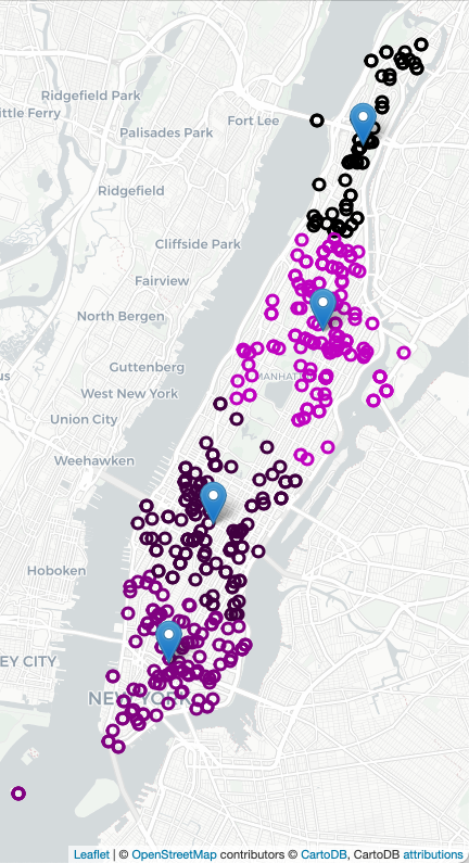
strategic placement of ambulance stations and overall allocation has been shown an effective approach. For example, here are all the calls for ambulances on 4 July 2021 in Manhattan (using Folium/Leaflet to create an interactive map):
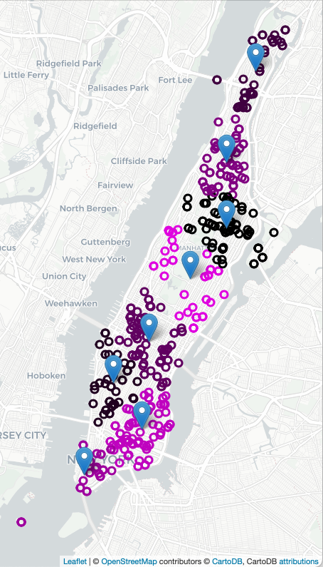
To decide on where to "pre-place" ambulances, we will use K-means clustering, where "K" is the number of ambulances available for that shift. For example, if there 2 ambulances available to be placed in Manhattan, we will look at previous ambulance calls for that shift and form 2 clusters and station each ambulance at the mean of the cluster. If two more ambulances become available, we can recompute the K-means algorithm for K=4, and place those 4 ambulances, each at the mean of the cluster found, and similarly for K=8:
The assignment is broken into the following functions to allow for unit testing:
For example, if we use the small dataset from 4 July 2021:
Let's add in the date and time features:
Let's add in the date and time features:
We can build a map with the calls for ambulances shaded by the time of the call:
We can also make maps with the computed clusters. We use the Another function can be used to filter the dataset by day of the week and time of day. For example, still working with the 4 July data set:
Let's next filter for early morning times:
Lastly, we can use the function showing a sharp drop-off to
Learning Objective: to enhance data cleaning skills and build understanding of clustering algorithms.
Available Libraries: pandas, datetime, numpy, sklearn, and core Python 3.6+.
Data Sources: 911 System Calls (NYC OpenData)
Sample Datasets:

make_df(file_name):
This function takes one input:
The data is read into a DataFrame. Rows that are have null values for the type description, incident date, incident time, latitute and longitude are dropped.
Only rows that contain file_name: the name of a CSV file containing 911 System Calls from OpenData NYC.
AMBULANCE as part of the TYP_DESC are kept. The resulting DataFrame is returned.
Hint: see DS 100: Chapter 13 for using string methods within pandas.
add_date_time_features(df):
This function takes one input:
An additional column df: a DataFrame containing 911 System Calls from OpenData NYC created by make_df.
WEEK_DAY is added with the day of the week (0 for Monday, 1 for Tuesday, ..., 6 for Sunday) of the date in INCIDENT_DATE is added.
Another column, INCIDENT_MIN, that takes the time from INCIDENT_TIME and stores it as the number of minutes since midnight. The resulting DataFrame is returned.
Hint: see Lecture 7 for using datetime methods with pandas, including computing the day of the week (of datetime objects) and the total seconds (of timedelta objects).
filter_by_time(df,days=None,times=[0,1439]):
This function takes three inputs:
Returns a DataFrame with entries restricted to weekdays in df: a DataFrame containing 911 System Calls from OpenData NYC.
days: a list of integers ranging from 0 to 6, representing the days of the week. The default value is None and is equivalent to the list containing all days:
[0,1,2,3,4,5,6].
times: a list of two non-negative integer values representing the range, inclusive, for the time, in minutes, that should be selected. The default value is [0,1439] which ranges from midnight (0 minutes) to (1439 representing 23:59 since 23 hours + 59 minutes = 23*60+59 minutes = 1439 minutes).
days (or all weekdays if None is given) and incident times in times inclusive (e.g. contains the endpoints).
compute_locations(df, num_clusters = 8, random_state = 2022):
This function takes three input:
Runs the KMeans model with df: a DataFrame containing 911 System Calls from OpenData NYC.
num_clusters: an integer representing the number of clusters. The default value is 8.
random_state: the random seed used for KMeans. The default value is 2022.
num_clusters on the latitude and longitude data of the provided DataFrame. Returns the cluster centers and predicted labels computed via the model.
compute_explained_variance(df, K =[1,2,3,4,5], random_state = 55):
This function takes three inputs:
Returns a list of the sum of squared distances of samples to their closest cluster center for each value of df: a DataFrame containing 911 System Calls from OpenData NYC.
K: a list of integers representing values for the number of clusters. The default value is [1,2,3,4,5].
random_state: the random seed used for KMeans. The default value is 55.
K. This can be computed manually or via the inertia_ attribute of the KMeans model.
would print:
df = make_df('NYPD_Calls_Manhattan_4Jul2021.csv')
print(df[['INCIDENT_TIME','TYP_DESC','Latitude','Longitude']])
Note that the original CSV file had over 5000 lines, only 459 of those were for ambulances calls. The indices were not reset and refer to the line numbers of the original file.
     INCIDENT_TIME                             TYP_DESC   Latitude  Longitude
7         00:01:51      AMBULANCE CASE: CARDIAC/OUTSIDE  40.724578 -73.992519
27        00:06:12       AMBULANCE CASE: CARDIAC/INSIDE  40.807719 -73.964240
51        00:12:12      AMBULANCE CASE: SERIOUS/TRANSIT  40.732019 -74.000734
53        00:12:38           AMBULANCE CASE: EDP/INSIDE  40.789348 -73.947352
54        00:12:38           AMBULANCE CASE: EDP/INSIDE  40.789348 -73.947352
...            ...                                  ...        ...        ...
5175      23:50:02         AMBULANCE CASE: WATER RESCUE  40.711839 -74.011234
5176      23:50:02         AMBULANCE CASE: WATER RESCUE  40.711839 -74.011234
5205      23:57:11  AMBULANCE CASE: UNCONSCIOUS/TRANSIT  40.732019 -74.000734
5211      23:57:59           AMBULANCE CASE: EDP/INSIDE  40.827547 -73.937461
5212      23:57:59           AMBULANCE CASE: EDP/INSIDE  40.827547 -73.937461

[459 rows x 4 columns]
would print:
df = add_date_time_features(df)
print(df[['INCIDENT_DATE','WEEK_DAY','INCIDENT_TIME','INCIDENT_MIN']])
Since all the incidents are from a single day (i.e. 4 July 2021) the INCIDENT_DATE WEEK_DAY INCIDENT_TIME INCIDENT_MIN
7 07/04/2021 6 00:01:51 1.850000
27 07/04/2021 6 00:06:12 6.200000
51 07/04/2021 6 00:12:12 12.200000
53 07/04/2021 6 00:12:38 12.633333
54 07/04/2021 6 00:12:38 12.633333
... ... ... ... ...
5175 07/04/2021 6 23:50:02 1430.033333
5176 07/04/2021 6 23:50:02 1430.033333
5205 07/04/2021 6 23:57:11 1437.183333
5211 07/04/2021 6 23:57:59 1437.983333
5212 07/04/2021 6 23:57:59 1437.983333
[459 rows x 4 columns]
[Finished in 2.294s]WEEK_DAY column has the same value (i.e. 6) for every row.
would print:
df_early_am = filter_by_time(df,times=[0,360])
print(df_early_am[['INCIDENT_DATE','WEEK_DAY','INCIDENT_TIME','INCIDENT_MIN']]) INCIDENT_DATE WEEK_DAY INCIDENT_TIME INCIDENT_MIN
7 07/04/2021 6 00:01:51 1.850000
27 07/04/2021 6 00:06:12 6.200000
51 07/04/2021 6 00:12:12 12.200000
53 07/04/2021 6 00:12:38 12.633333
54 07/04/2021 6 00:12:38 12.633333
... ... ... ... ...
1041 07/04/2021 6 05:08:49 308.816667
1068 07/04/2021 6 05:21:49 321.816667
1075 07/04/2021 6 05:24:21 324.350000
1079 07/04/2021 6 05:28:13 328.216667
1111 07/04/2021 6 05:41:34 341.566667
[76 rows x 4 columns]
displayed above. Note that we used the time to shade the incidents. The popups provide the exact time as well as the description.
import folium
import matplotlib.colors
def cc(minute,scale):
    return(matplotlib.colors.to_hex( (minute/scale,0,minute/scale) ))

m = folium.Map(location=[40.7678,-73.9645],zoom_start=13,tiles="cartodbpositron")
df.apply( lambda row: folium.CircleMarker(location=[row["Latitude"], row["Longitude"]],
                                        radius=5, popup=(row['INCIDENT_TIME']+": "+row['TYP_DESC']),
                                        color=cc(row['INCIDENT_MIN'],2000))
                                        .add_to(m) ,
        axis=1)
m.save('4_July_map.html')compute_locations function with different values of num_clusters. Since we are repeating the same actions for K = 2, 4, 6, we wrote a helper function to create the HTML maps:
Screenshots of the maps are displayed above.
def make_map(df, num_clusters, out_file):
    centers,labels = compute_locations(df,num_clusters = num_clusters)
    df_map = df[ ['Latitude','Longitude','INCIDENT_TIME','INCIDENT_MIN','TYP_DESC'] ]
    df_map = df_map.assign(Labels = labels)
    m = folium.Map(location=[40.7678,-73.9645],zoom_start=13,tiles="cartodbpositron")
    df_map.apply( lambda row: folium.CircleMarker(location=[row["Latitude"], row["Longitude"]],
                                        radius=5, popup=(row['INCIDENT_TIME']+": "+row['TYP_DESC']),
                                        color=cc(row['Labels'],num_clusters))
                                        .add_to(m), axis=1)
    for i in range(num_clusters):
        x,y = centers[i]
        folium.Marker(location=[x,y],popup = "Cluster "+str(i)).add_to(m)
    m.save(out_file)

make_map(df,2,'map_4_July_2clusters.html')
make_map(df,4,'map_4_July_4clusters.html')
make_map(df,8,'map_4_July_8clusters.html')
This will return an empty DataFrame since only 4 of July in this data set (which was a Sunday and we filtered for 0 or Monday):
df_mondays = filter_by_time(df, days = [0])
print(df_mondays)Empty DataFrame
Columns: [CAD_EVNT_ID, CREATE_DATE, INCIDENT_DATE, INCIDENT_TIME, NYPD_PCT_CD, BORO_NM, PATRL_BORO_NM, GEO_CD_X, GEO_CD_Y, RADIO_CODE, TYP_DESC, CIP_JOBS, ADD_TS, DISP_TS, ARRIVD_TS, CLOSNG_TS, Latitude, Longitude, WEEK_DAY, INCIDENT_MIN]
Index: []
would print:
df_early_am = filter_by_time(df,times=[0,360])
print(df_early_am[['INCIDENT_DATE','WEEK_DAY','INCIDENT_TIME','INCIDENT_MIN']]) INCIDENT_DATE WEEK_DAY INCIDENT_TIME INCIDENT_MIN
7 07/04/2021 6 00:01:51 1.850000
27 07/04/2021 6 00:06:12 6.200000
51 07/04/2021 6 00:12:12 12.200000
53 07/04/2021 6 00:12:38 12.633333
54 07/04/2021 6 00:12:38 12.633333
... ... ... ... ...
1041 07/04/2021 6 05:08:49 308.816667
1068 07/04/2021 6 05:21:49 321.816667
1075 07/04/2021 6 05:24:21 324.350000
1079 07/04/2021 6 05:28:13 328.216667
1111 07/04/2021 6 05:41:34 341.566667
[76 rows x 4 columns]compute_explained_variance to assess the best number of clusters:
will display:
k_vals = list(range(1,20))
ev = compute_explained_variance(df,K=k_vals)
sns.lineplot(k_vals,ev)
plt.title('Explained Variance for KMeans for Manhattan, 4 July 2021')
plt.show()

K=5 that quickly flattens, showing that additional clusters, beyond 10, do not significantly improve the average distance to the assigned means. This suggests that a reasonable number of clusters is around 8.