CSci 39542 Syllabus    Resources    Coursework

Program 11: Digit Dimensions
CSci 39542: Introduction to Data Science
Department of Computer Science
Hunter College, City University of New York
Spring 2022

---

Classwork    Quizzes    Homework    Project   

---

---

Program Description

Program 11: Digit Dimensions.   Due noon, Thursday, 29 April.
Learning Objective: to increase facility with standard linear algebra approaches and strengthen understanding of intrinistic dimensions of data sets via exploration of the classic digits dataset).
Available Libraries: pandas, numpy, pickle, sklearn, and core Python 3.6+.
Data Sources: MNIST dataset of hand-written digits, available in sklearn digits dataset.
Sample Datasets: sklearn digits dataset.

In Lecture 22 and Chapter 26, we applied Principal Components Analysis as a dimensionality reduction technique and used scree plots to provide a visualization of the captured variance. This assignment continues our analysis of the sklearn digits dataset, focusing on visualization and intrinsic dimenion of the data. In addition, we will write a function that allows the user to explore how many dimensions are needed to see the underlying structure of images from the sklearn digits dataset (inspired by Python Data Science Handbook: Section 5.9 (PCA)).

As in Program 10, we can view our images as "flattened" 1D arrays of length 64. As discussed in Python Data Science Handbook: Section 5.9, we can view the images as sums of the components. If we let x1 = [1 0 ... 0], x2 = [0 1 0 ... 0], ..., x64 = [0 ... 0 1] (vectors corresponding to the axis), then we can write our images, im = [i1 i2 ... i64], as: im = x1*i1 + x2*i2 + x3*i3 + ... + x64*i64. For example, if we take the first entry from the dataset:

[ 0.  0.  5. 13.  9.  1.  0.  0.  0.  0. 13. 15. 10. 15.  5.  0.  0.  3. 15.  2.  0. 11.  8.  0.  0.  4. 12.  0.  0.  8.  8.  0.  0.  5.  8.  0.  0.  9.  8.  0.  0.  4. 11.  0.  1. 12.  7.  0.  0.  2. 14.  5. 10. 12.  0.  0.  0.  0.  6. 13. 10.  0.  0.  0.]

We can write it as:

im = x1*i1 + x2*i2 + x3*i3 + ... + x64*i64
   = x1*0  + x2*0  + x3*5  + ... + x64*0

plugging in the values for a given image (in this case the first image in the dataset) into the equation.

In a similar fashion, we can represent the image in terms of the axis,c1, c2, ... c64, that the PCA analysis returns:

im = mean + c1*i1 + c2*i2 + ... + c64*i64

since the axis of PCA are chosen so that the first one captures the most variance, the second the next most, etc. The later axis capture very little variance and likely add litte to the image. For technical reasons, we include the mean (the reason is similar to when we "center" multidimensional data at 0). This can be very useful for reducing the dimension of the data set, for example, here is the first image from above on the left:

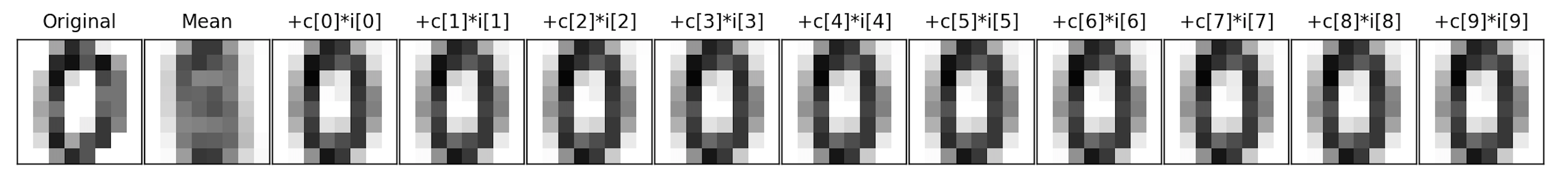
The next image is the overall mean, and each subsequent image is adding another component to the previous. For this particular scan, the mean plus its first component is enough to see that it's a 0.

In your program, include the following functions from Program 10. You may use your earlier function or the Program 10 solution available on Blackboard:

• select_data(data, target, labels = [0,1]): This function takes as three input parameters:
  • data: a numpy array that includes rows of equal size flattened arrays,
  • target a numpy array that contains the labels for each row in data.
  • labels: the labels from target that the rows to be selected. The default value is [0,1].
  Returns the rows of data and target where the value of target is in labels.

And write the following new functions:

• run_pca(xes): This function takes as one input parameter:
  • xes: a numpy array that includes rows of equal size flattened arrays,
  It fits a model of sklearn.decomposition.PCA to the xes. The function returns the model and the transformed values.
• capture_85(mod): This function takes as one input parameter:
  • mod: a model of sklearn.decomposition.PCA that has been fitted to a dataset.
  From the array of the amount of varianace of each component, (stored in mod.singular_values_), compute fraction of the variance of each component. That is, if sv = mod.singular_values_, then s=sv**2/sum(sv**2) (see Chapter 26.3.1.1 Captured Variance and Scree Plots). Returns the number of elements needed to capture more than 85% of the variance. For example, if sv is:

  array([585.57, 261.06, 166.31,  57.14,  48.16,  39.79,  31.71,  28.91,
          24.23,  22.23,  20.51,  18.96,  17.01,  15.73,   7.72,   4.3 ,
           1.95,   0.04])

  then s is

  array([0.76, 0.15, 0.06, 0.01, 0.01, 0.  , 0.  , 0.  , 0.  , 0.  , 0.  ,
         0.  , 0.  , 0.  , 0.  , 0.  , 0.  , 0.  ])

  The first component captures 76% of the variance which is lower than that 85% threshold. The first and second components capture (76+15)% = 91% of the variance, so, your function would return 2.
• average_eigenvalue(mod): This function takes as one input parameter:
  • mod: a model of sklearn.decomposition.PCA that has been fitted to a dataset.
  For the mod, computes the average of the eigenvalues (i.e. the average of sv = mod.singular_values_) and returns the number of elements greater than the average. See sklearn.decomposition.PCA for attributes of the model.
• approx_digits(mod, img, numComponents=8): This function has three inputs:
  • mod: a model of sklearn.decomposition.PCA that has been fitted to a dataset.
  • img: a flattened image from the dataset.
  • numComponents: the number of components used in the approximation. Expecting a value between 0 and 64. The default value is 8.
  The function transforms the image, img, and uses the resulting coefficents to compute an approximation of the image. The approximation image (flattened array) is the mean plus the sum of the first numComponents terms (i.e. coefficients[i] * components[i] where the coefficients are returned from the transform and components are an array of the components computed by PCA() analysis). Note that the mean of the dataset does not have to be computed since it is stored as an attribute of the models of PCA(). Returns the computed approximation image as a flattened array. Hint: see the discussion in DS Handbook 5.09 (PCA) and in Lecture 21.

Let's run through a few examples. We can start with our binary digits from Program 10:

from sklearn import datasets
digits = datasets.load_digits()
n_samples = len(digits.images)
data = digits.images.reshape((n_samples, -1))
target = digits.target
print(f'The targets for the first 5 entries: {target[:5]}')
bin_dig, bin_tar = select_data(data,digits.target)
print(f'The targets for the first 5 binary entries: {bin_tar[:5]}')

which prints:

pca = PCA().fit(digits.data)
The targets for the first 5 binary entries: (0, 1, 0, 1, 0)

Using our function from Program 10, we can select the binary digits and then fit the PCA model to those. Our function returns the model as well as the transformed values:

import matplotlib.pyplot as plt
bin_data,bin_target = select_data(data,target)
bin_mod, bin_proj = run_pca(bin_data)
scatter = plt.scatter(bin_proj[:, 0], bin_proj[:, 1], c=bin_target, alpha=0.5,
            cmap=plt.cm.get_cmap('rainbow', 10))
plt.title('PCA for digits')
plt.xlabel('Component 1')
plt.ylabel('Component 2')
plt.legend(*scatter.legend_elements())
plt.show()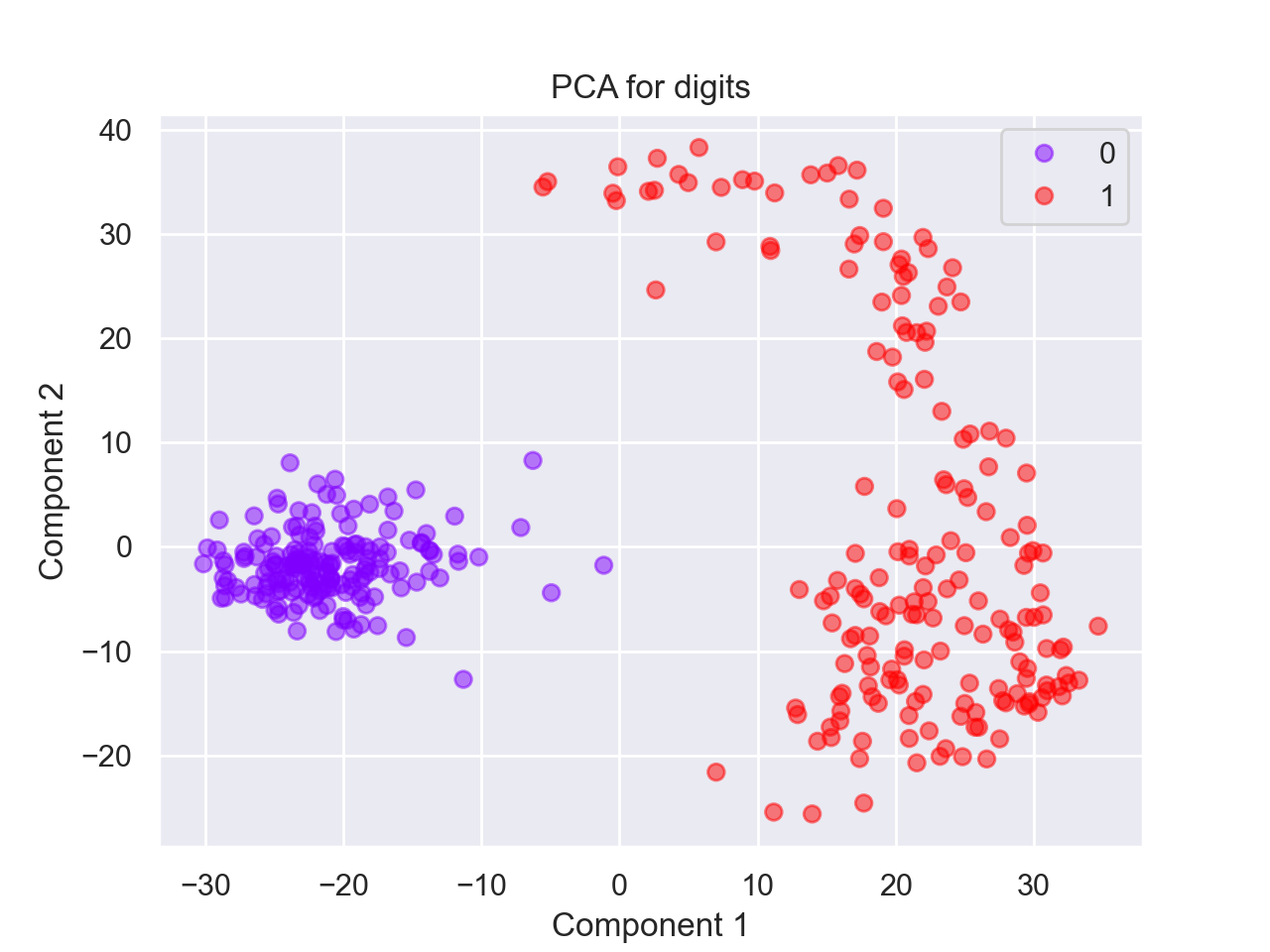

The resulting image shows two distinct clusters for the images labeled 0 and those labeled 1:

We can fit the model to all the digits:

all_mod, all_proj = run_pca(data)
scatter = plt.scatter(all_proj[:, 0], all_proj[:, 1], c=digits.target, alpha=0.5,
            cmap=plt.cm.get_cmap('rainbow', 10))
plt.title('PCA for digits')
plt.xlabel('Component 1')
plt.ylabel('Component 2')
plt.legend(*scatter.legend_elements())
plt.show()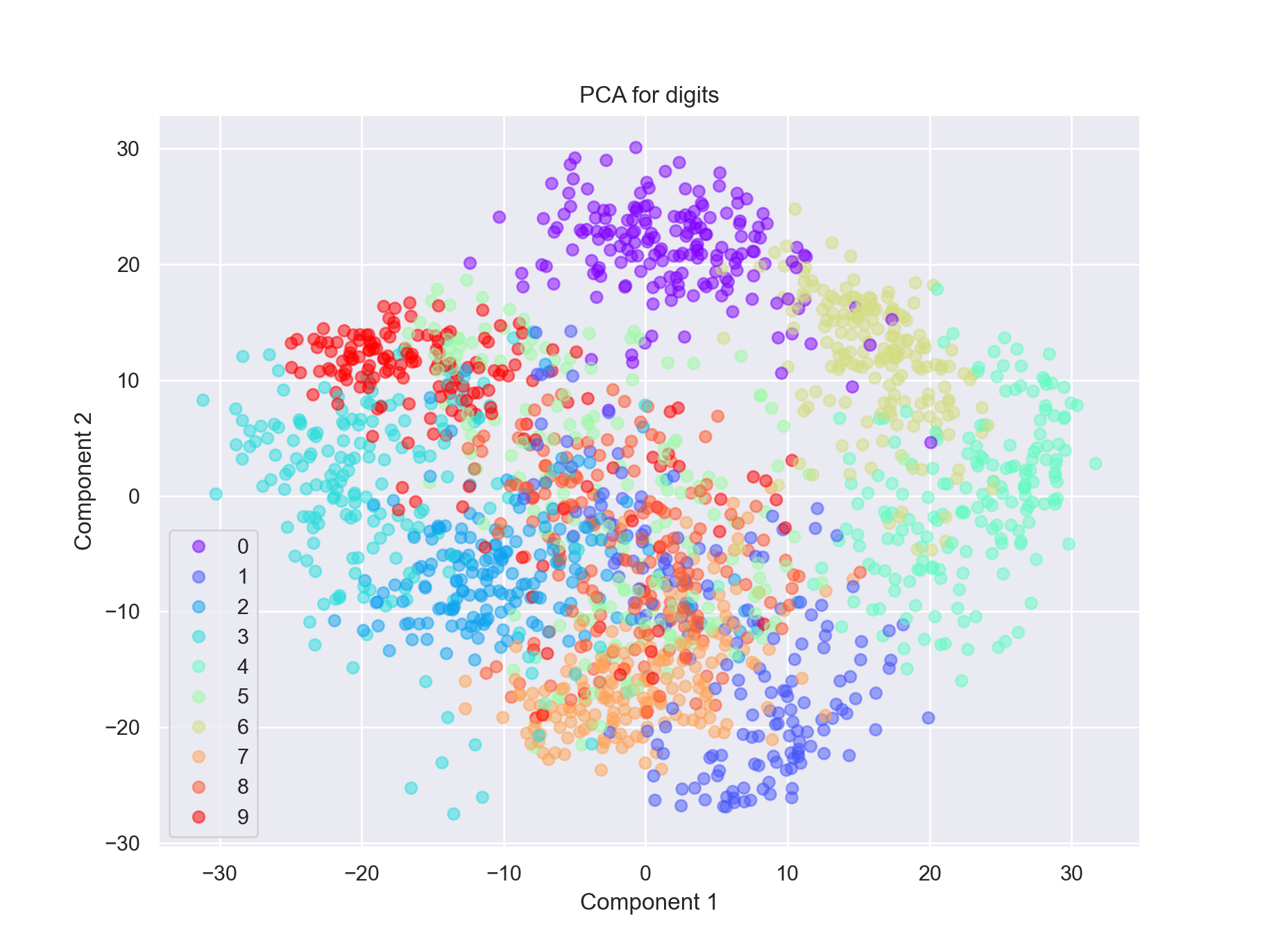

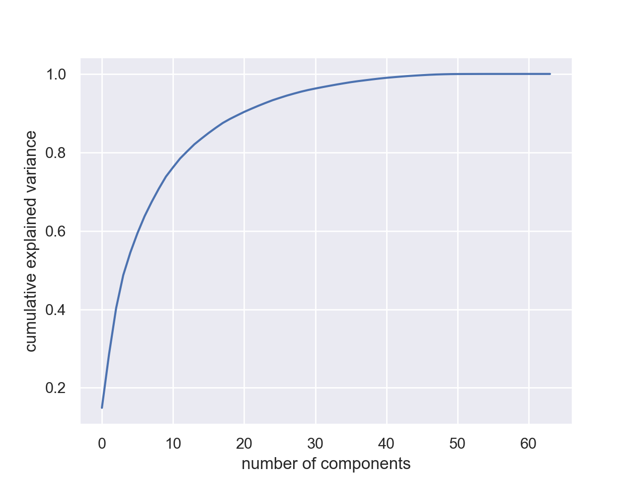
When looking at the complete data set, the projection to the first coordinates has some grouping of the images by labels:

Plotting the explained variance ratio of our model:

import numpy as np
plt.plot(np.cumsum(all_mod.explained_variance_ratio_))
plt.xlabel('number of components')
plt.ylabel('cumulative explained variance')
plt.show()

The resulting image shows that much of the variance is captured by the first 10 components:

We can use our functions to look at ways to measure this, via the captured variance and average eigenvalues:

np.set_printoptions(suppress=True)  #Turn off scientific notation
sv = all_mod.singular_values_
print(f'The singular values are: {sv}')
print(f'The fraction variance: {sv**2/sum(sv**2)}')
print(f'The number of components needed to capture 85% of the variance is {answer.captures85(all_mod)}.')
print(f'The number of eigenvalues larger than the average is {answer.averageEigenvalue(all_mod)}.')

prints out the explained variance as well as the numbers computed by our functions:

The singular values are: [567.0065665  542.25185421 504.63059421 426.11767608 353.3350328
 325.82036569 305.26158002 281.16033073 269.06978193 257.82395143
 226.31879719 221.5148324  198.33071545 195.70013887 177.9762712
 174.46079067 168.72787641 164.15849219 148.23330876 139.83132462
 138.58443271 131.1882069  128.72691665 124.93159016 122.57503405
 113.44487728 111.48027133 105.46348813 102.80780243  96.22856616
  89.81296469  87.33494649  85.25960437  84.15671337  81.58936529
  79.64200462  74.43047136  70.12195688  69.27559227  67.56406817
  64.03315896  58.52697795  57.12818557  55.09243185  50.17909986
  48.1749428   45.62286487  40.89585718  34.68503519  29.5461187
  21.28899661  13.34460261  10.64814019  10.44437712   8.44041164
   5.18181553   3.90097916   2.55109635   1.51445826   1.08979014
   0.86043771   0.           0.           0.        ]
The fraction variance: [0.14890594 0.13618771 0.11794594 0.08409979 0.05782415 0.0491691
 0.04315987 0.03661373 0.03353248 0.03078806 0.02372341 0.02272697
 0.01821863 0.01773855 0.01467101 0.01409716 0.01318589 0.01248138
 0.01017718 0.00905617 0.00889538 0.00797123 0.00767493 0.00722904
 0.00695889 0.00596081 0.00575615 0.00515158 0.0048954  0.00428888
 0.00373606 0.00353274 0.00336684 0.0032803  0.00308321 0.00293779
 0.00256589 0.00227742 0.00222278 0.0021143  0.00189909 0.00158653
 0.0015116  0.00140579 0.00116622 0.00107493 0.00096405 0.00077463
 0.00055721 0.00040433 0.00020992 0.00008248 0.00005251 0.00005052
 0.000033   0.00001244 0.00000705 0.00000301 0.00000106 0.00000055
 0.00000034 0.         0.         0.        ]
The number of components needed to capture 85% of the variance is 17.
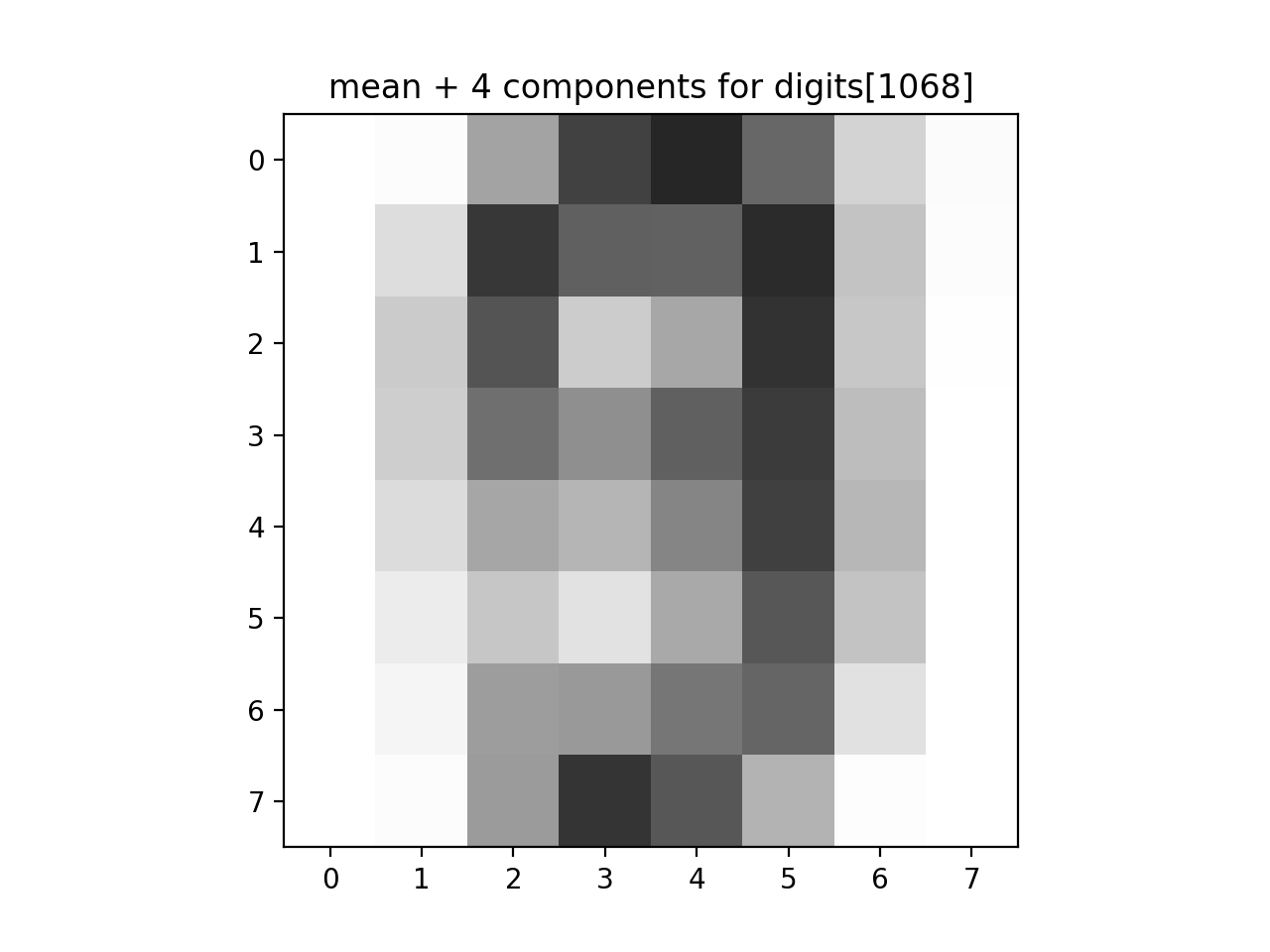
The number of eigenvalues larger than the average is 23.

Lastly, let's look at how many components are needed to recover a given image:

plt.imshow(all_mod.mean_.reshape(8, 8), cmap='binary', interpolation='nearest', clim=(0, 16))
plt.title("Mean for digits")
plt.show()

print(f'The original image: {data[1068]}.')

approx_answer = approx_digits(all_mod, all_proj[1068], numComponents=4)
print(f'The first 4 components: {approx_answer}')
plt.imshow(approx_answer.reshape(8, 8), cmap='binary', interpolation='nearest', clim=(0, 16))
plt.title("mean + 4 components for digits[1068]")
plt.show()

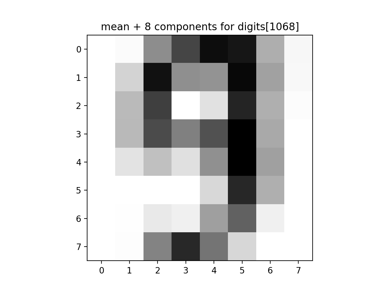
approx_answer = approx_digits(all_mod, all_proj[1068], numComponents=8)
print(f'The first 8 components: {approx_answer}')
plt.imshow(approx_answer.reshape(8, 8), cmap='binary', interpolation='nearest', clim=(0, 16))
plt.title("mean + 8 components for digits[1068]")
plt.show()

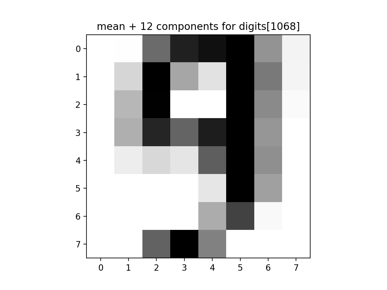
approx_answer = approx_digits(all_mod, all_proj[1068], numComponents=12)
print(f'The first 12 components: {approx_answer}')
plt.imshow(approx_answer.reshape(8, 8), cmap='binary', interpolation='nearest', clim=(0, 16))
plt.title("mean + 12 components for digits[1068]")
plt.show()

Below we have the mean of all the images and the result of adding the first 4 components, the first 8 components, and the first 12 components for data[1068]: